Setting Up your Environment

---

If you want to follow the textbook by running the code presented in here but don’t know how to get started, you are in luck! Below is a step by step description of how to get started.

If you’re comfortable working on a terminal window, the Summary section below gives the minimal necessary steps. For more details, see sections 1-3 below.

0. Summary

• Install Miniconda

• In a terminal window, create a new environment

  conda create --name <my-env> python=3

• Activate new environment

  conda activate <my-env>

• Install Jupyter Notebook

  pip install notebook

• Install Qiskit

  • On macOS (zsh):

    pip install 'qiskit[visualization]'

  • On Windows, Linux (bash):

    pip install qiskit[visualization]

• Install Qiskit Aer

  pip install qiskit-aer

• Install Qiskit’s IBM Runtime

  pip install qiskit-ibm-runtime

• Verify your Environment

1. Install Minicoda

Before installing any of the necessary Python packages, it is highly recommended to use what is known as a virtual environment manager. This allows us to have a separate environment where we can specify the version of Python we want to use and the dependencies (packages) we needed for our project. Two popular options for Python environments are venv and conda. Here we will use the latter.

To get conda up and running we need to install Miniconda, which can be done by downloading the installer corresponding to your operating system.

Once the download completes, run the installer and follow the directions to specify where you want things to reside.

• macOS users: it is easier to download and install the pkg version over the bash version since it comes with a visual user interface.
  
  

• Windows users: if this is your first installation of a python distribution, it is highly recommended you check the box that says “Add Miniconda3 to my PATH environment variable”

2. Create and Activate a Virtual Environment

With Miniconda installed, open a terminal window if you are on MacOs or Linux. If you are on Windows, open the Anaconda Prompt (Anaconda3). You can find it by clicking on the Windows logo key and typing Anaconda.

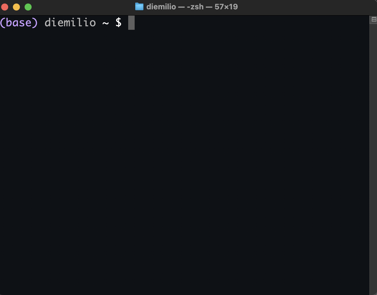
The command line should display that you’re on the base environment:

To create a new virtual environment type and run:

conda create --name <my-env> python=3

Replace <my-env> with whatever name you want to use for your environment.

When asked if you want to proceed, type y. This will create a new environment equiped with the latest stable version of Python.

Lastly, make sure to activate your environment before proceeding with any of the package installations by running:

conda activate <my-env>

where, again, <my-env> is the name you selected for your environment.

3. Install Necessary Python Packages

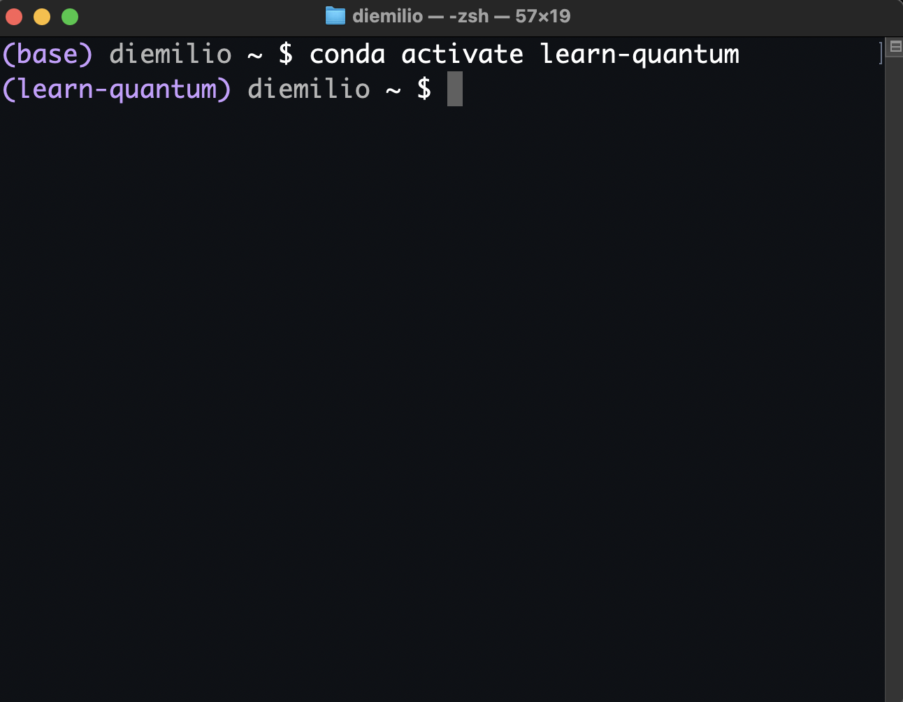
Again, make sure you have activated the new environment before proceeding with any of the installations. The environment name should be displayed on the terminal command line right before your username. In the example below, we have activated an environment named learn-quantum:

Once in the right environment, we can start installing the necessary packages to execute the code in this textbook. Here’s the list of packages with a short explanation of why we need them:

1. Jupyter Notebook

   Each chapter of this textbook is written in a Jupyter Notebook, which allows us to have both markdown cells to, for example, write text and equations that can be rendered in LaTeX, and code cells to write and execute Python code. Therefore, installing this package will allow you to download the textbook and run the cells, or simply copy and paste the code for execution. To install this package, run the following line in the terminal prompt:

   pip install notebook
   

2. Qiskit

   Qiskit is currently considered to be the most popular Python package for the implementation, simulation, and execution of quantum circuits. Therefore this is the main package we will use throughout this textbook. Installing qiskit also installs its dependencies. In other words, the qiskit installation adds other packages that we will need throughout the textbook, such as NumPy, SymPy, Matplotlib, among many others.

   If you have a recent version of macOS (or Linux zsh shell), run the following line in the terminal prompt to install qiskit (with all of its required depedencies):

   pip install 'qiskit[visualization]'
   

   If instead you are running the Annaconda Prompt in Windows, or are in a Linux bash shell, then run:

   pip install qiskit[visualization]
   

3. Qiskit Aer

   Qiskit Aer is a separate package that contains high-performance noisy simulators for Qiskit. We will be using these simulators in later chapters where we will cover noise. To install this package, run the following line in the terminal prompt:

   pip install qiskit-aer
   

4. Qiskit IBM Runtime

   The Qiskit IBM Runtime package contains the functions needed to access IBM’s quantum processing units (QPUs). In other words, this package will allow us to connect to real quantum hardware, which we might do in some chapters of the textbook. To install this package, run the following line in the terminal prompt:

   pip install qiskit-ibm-runtime
   

   NOTE: To be able to run your quantum programs in IBM’s hardware, you need an IBM Quantum account. You can find help on how to set this up right after you’re done verifying your environment by following the instructions in the Configuring Qiskit chapter of this textbook.

4. Verify your Environment

To verify everything was installed properly, open a Jupyter Notebook by running in the terminal prompt:

jupyter notebook

Select the folder where you want to save your notebook, and on the top right, click “New” and select “Python 3”.

Copy and paste the code below on the first cell of the notebook and make sure it runs correctly. Do not worry if you don’t understand the code, we’re just verifying all libraries are accessible. This code does not verify if qiskit-ibm-runtime package is properly installed, but we will cover this in section 1 of the next chapter.

If you run into issues, you can post questions in the discussions section, but make sure to follow the guidelines.

import numpy as np
from qiskit import QuantumCircuit, transpile
from qiskit.quantum_info import Statevector
from qiskit.visualization import plot_distribution
from qiskit_aer import AerSimulator

simulator = AerSimulator()

qc = QuantumCircuit(2,2)
qc.rx(np.pi/2,1)
qc.cx(1,0)
print("Statevector:")
display(Statevector(qc).draw('latex'))

qc.measure([1,0],[1,0])

print("Circuit:")
display(qc.draw('mpl'))

qc_t = transpile(qc, simulator)
counts = simulator.run(qc, shots=2**10).result().get_counts()

print("Probability Distribution:")
plot_distribution(counts)

Statevector:

\[\frac{\sqrt{2}}{2} |00\rangle- \frac{\sqrt{2} i}{2} |11\rangle\]

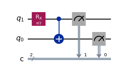
Circuit:

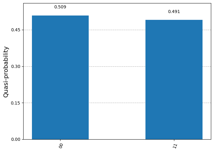
Probability Distribution: