Grover’s Algorithm

---

Grover’s algorithm, introduced by Lov Grover in 1996, marked the second major discovery of a quantum algorithm with potential practical applications, appearing only a few years after Shor’s factoring algorithm. However, unlike Shor’s exponential speedup, Grover’s algorithm provides only a polynomial advantage (specifically, quadratic) over the best known classical approaches [Grover96]. In other words, for certain problems that require \(N\) steps classically, Grover’s algorithm can find a solution with high probability in roughly \(\sqrt{N}\) steps.

Grover’s algorithm is also known as the quantum search algorithm, as it addresses the problem of finding the inputs to an arbitrary function that evaluate to some specified output value. More precisely, the class of problems it solves can be formulated as instances of an unstructured search, where given a Boolean function \(f: \{0, 1\}^n \longmapsto \{0, 1\}\), the goal is to find all inputs \(x \in \{0, 1\}^n\) that evaluate to \(f(x) = 1.\)

A popular example used to describe Grover’s algorithm is the task of searching through a phone book to find the person associated with a specific phone number. This is a challenging task because, even though names are listed alphabetically, phone numbers themselves are unordered. So, if there are a total of \(N\) entries, a classical search may require checking each entry one by one until the number we’re looking for is found. In the worst case, this requires going over each of the \(N\) values. And for multiple of these searches, it takes on average \(N/2\) tries. In contrast, Grover’s algorithm can solve this problem by querying the list only \(\sqrt{N}\) times. However, as with the other quantum algorithms we’ve discussed so far, Grover’s algorithm requires encoding the problem of interest into a unitary oracle \(U_f.\) For a purely classical search task (such as scanning a phone book), constructing the function \(f(x)\) needed to build \(U_f\) would itself require examining the entire list of numbers ahead of time. Therefore, Grover’s algorithm offers no practical advantage in this particular use case. It is then crucial to recognize that, even though this example is helpful from a pedagogical standpoint, Grover’s algorithm is of practical use only when the function \(f(x)\) can be implemented and encoded into \(U_f\) in an efficient manner. An important task where this condition holds is in the circuit satisfiability problem, which we will discuss in a future chapter.

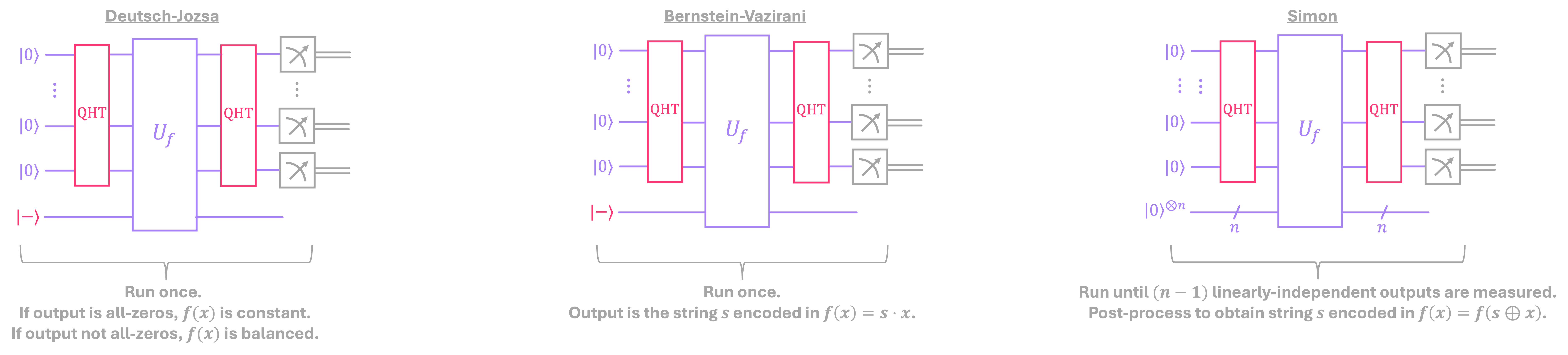
For convenience, we begin by formulating the unstructured search problem under the assumption that the unitary \(U_f\) is simply given to us. This mirrors our treatment of the Deutsch–Jozsa, Bernstein–Vazirani, and Simon algorithms, where, given access to \(U_f,\) we compare the number of queries required when it is evaluated using only classical inputs with the number required when quantum operations are allowed.

1. Classical Approach

A good starting point is to consider a function \(f(x)\) for which only one unknown value of \(x\) evaluates to \(1\) (we will generalize the problem for \(M\) unknown values in section 3). It is common to refer to this value as a marked element. Below is an example of a function for which the marked element is \(m = 101:\)

\[\begin{split} \begin{split} \begin{aligned} f(000) &= 0 \\ f(001) &= 0 \\ f(010) &= 0 \\ f(011) &= 0 \\ f(100) &= 0 \\ f(101) &= 1 \\ f(110) &= 0 \\ f(111) &= 0 \end{aligned} \end{split} \end{split}\]

Let’s use python to create a function \(f(x),\) which evaluates to \(1\) for a random marked element \(m.\)

import numpy as np

def fx_single_m(n):
    N = 2**n
    fx_lst = [0]*N
    
    m_int = np.random.randint(N)
    fx_lst[m_int] = 1
    
    return fx_lst, m_int

n = 3 # number of bits

fx_lst, m_int = fx_single_m(n)
m = np.binary_repr(m_int,n)

print(f'Outcomes for m = {m}\n')
print('x',' '*(n), 'f(x)')

for x_int, fx_int in enumerate(fx_lst):
    x = np.binary_repr(x_int,n)
    fx = np.binary_repr(fx_int,1)
    
    print(x, ' ', fx)

Outcomes for m = 011

x     f(x)
000   0
001   0
010   0
011   1
100   0
101   0
110   0
111   0

As mentioned above, the only way of finding a marked element classically is by evaluating \(f(x)\) for each input \(x\) until we get an output equal \(1\). The probability of succeeded after trying \(r\) different inputs is simply given by the ratio between the number of tries and the total number of possible inputs:

\[\mathbb{P}_{\text{success}} = \frac{r}{2^n} .\]

Let us now encode \(f(x)\) into a unitary \(U_f\) using qiskit:

from qiskit import QuantumCircuit, QuantumRegister, transpile
from qiskit_aer import AerSimulator

def Uf_one_marked(n):
    N = 2**n
    m_int = np.random.randint(N)
    m = np.binary_repr(m_int,n)
    
    qc_bb = QuantumCircuit(n+1, name=' $U_f$ (Oracle)')
    qc_bb.mcx(list(range(1,n+1)),0, ctrl_state=m)
    
    return qc_bb, m

# Draw example circuit for f(x) = 1 when x is the marked element m.
n = 4
bb, m = Uf_one_marked(n)

xr = QuantumRegister(n, name='x')
yr = QuantumRegister(1, name='y')

qc = QuantumCircuit(yr,xr)
qc.append(bb,range(n+1))

print(f'circuit that encodes f(x)=1 for x = {m}')
qc.decompose().draw()

circuit that encodes f(x)=1 for x = 0100

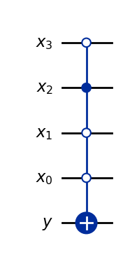
As can be seen, the black box circuit is very simple. It consists of an \(MCX\) gate for which the controls activate the \(X\) gate only when the input \(x = m.\) We can then run a simulation for one unknown marked element and see how many accesses to \(U_f\) it takes to find it:

n = 5                          # Length (in bits) of marked element
N = 2**n                       # Number of possible values x can take
simulator = AerSimulator()

bb, m = Uf_one_marked(n)  # Generate black box and secret string

for x_in in range(N):
    
    qc = QuantumCircuit(n+1,1)
    qc.prepare_state(x_in,range(1,n+1))
    qc.append(bb,range(n+1))
    qc.measure(0,0)

    qc_t = transpile(qc, simulator)
    job = simulator.run(qc_t, shots=1, memory=True)  # Run one simulation per black box 

    fx = job.result().get_memory()[0]

    if fx == '1':
        break
        
print(f'marked element: {m}')
print(f'found after: {x_in} tries out of {N}')

marked element: 10111
found after: 23 tries out of 32

The plot below shows the results of running the simulation above a large number of times for random marked elements of length \(n = 5\). As can be seen, it requires going over all \(N\) elements to guarantee finding the marked element with \(100 \%\) probability. Furthermore, the expected probability of success increases as \(r/2^n.\) This implies that, it takes \(r = 2^n/2 = 2^{n-1}\) tries to find the marked element \(m\) with more than \(50 \%\) probability, which for \(n = 5,\) is \(r = 16:\)

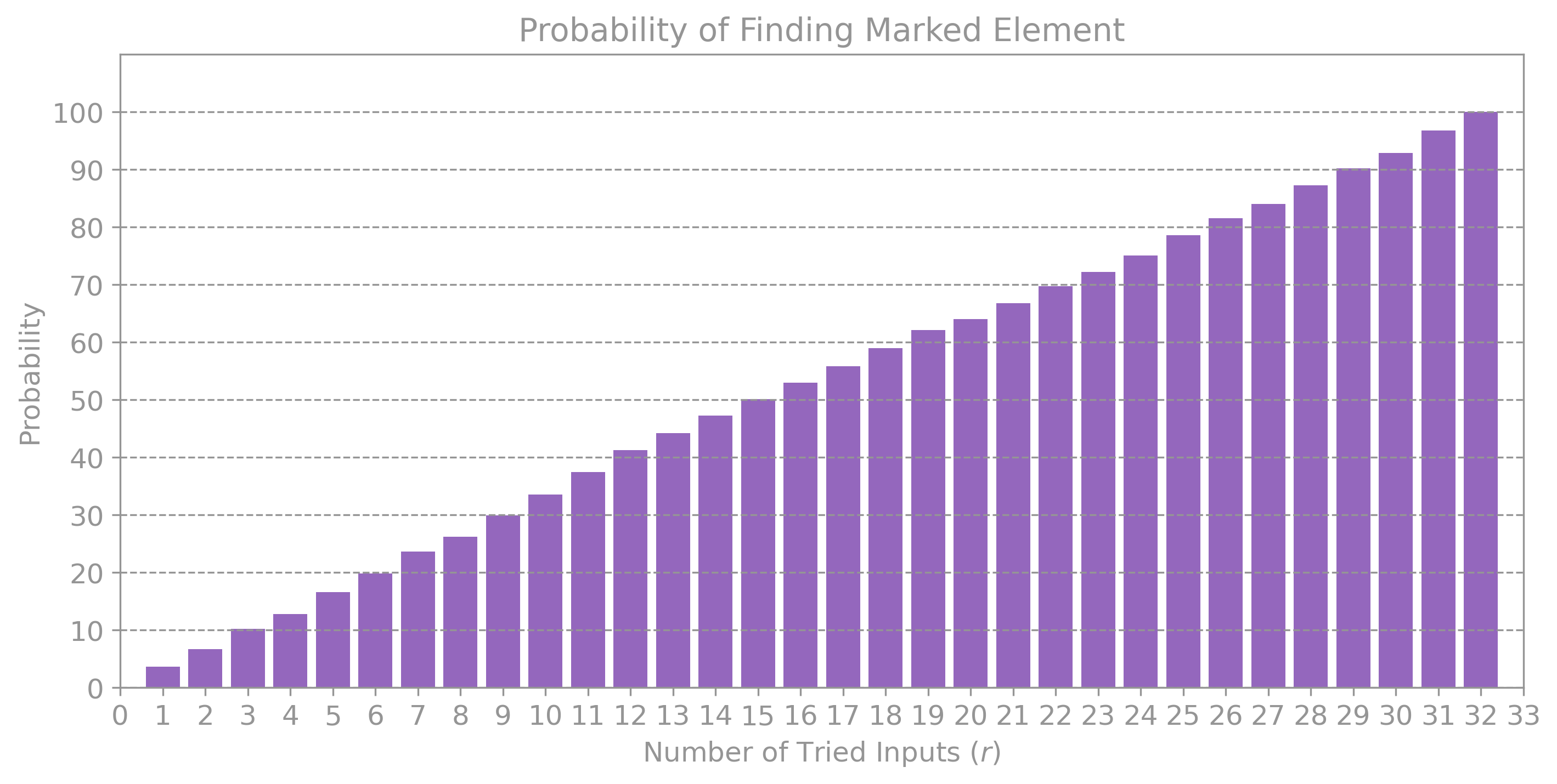
The main takeaway here is that, as the number of possible inputs \(N = 2^n\) increases, the number of times we need to access the oracle \(U_f\) to find \(m\) with high probability also increases linearly with \(N.\)

2. Quantum Approach

Grover’s algorithm follows a similar set of steps to those we’ve used in previous algorithms, where we:

1. Place all inputs in an equal superposition using the Quantum Hadamard Transform \((\text{QHT}).\)

2. Evaluate a function of interest \(U_{f(x)}\) (which encodes our problem) over the equal superposition state.

3. Perform constructive/destructive interference using the \(\text{QHT}\).

4. Measure the top register to extract relevant information about our solution.

However, as we will see next, in Grover’s algorithm the interference step is performed by a unitary different from the \(\text{QHT}.\) The role of this operation is to amplify the probability of measuring the marked element \(m.\) Moreover, the amount of amplification achieved in each iteration depends on the total number of elements \(N\), meaning that the circuit must be applied repeatedly to maximize the probability of measuring \(m\) in the top register. What’s critical though, is that the number of repetitions (and therefore the number of calls to \(U_f\)) scales proportional to \(\sqrt{N},\) representing a quadratic improvement over the classical approach described in section 1, which required a number of calls to \(U_f\) on the order of \(N.\)

2.1 Quantum Circuit

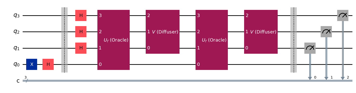
The image below shows a general sketch of the quantum circuit used in Grover’s algorithm.

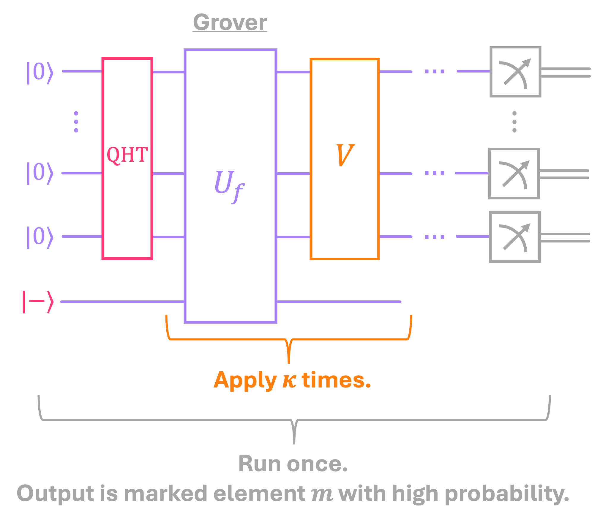
Like with previous algorithms, we start by placing the input in an equal superposition over all \(N = 2^n\) possible values of \(x \in \{0, 1\}^n.\)

Next, we perform quantum function evaluation, where \(U_f\) encodes the function \(f(x)\), which equals \(1\) only for the input \(x = m.\) As mentioned above, the function evaluation step is now followed by a unitary \(V,\) commonly known as Grover’s Amplification or Diffusion operator. \(V\) still performs constructive/destructive interference just like the \(\text{QHT}\) does in other algorithms, but in a more subtle way. \(V\) is responsible of amplifying the probability amplitude associated with the marked element \(m\), and diffusing the amplitudes of all other elements.

An important aspect of this amplification step is that, since the amount by which the probability of interest increases depends on the total number of elements in the search space, we must repeat the application of \(U_f\) and \(V\) a certain number of times \(\kappa\) to guarantee that the measured output is the marked element \(m\) with high probability.

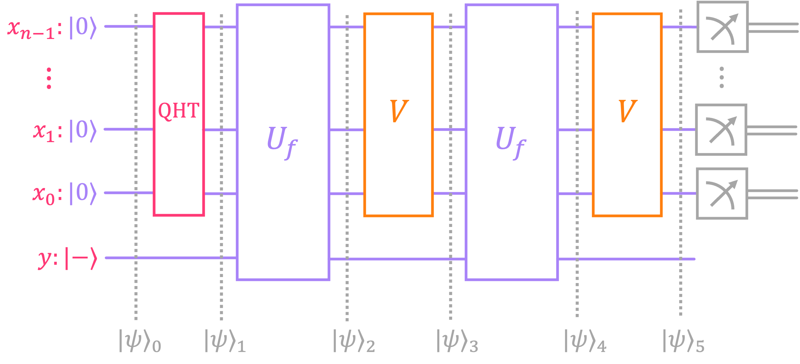
Let’s go over each circuit step to understand the role of the diffuser \(V,\) and why \(U_f\) and \(V\) might need to be repeated more than once before measurement. We will accompany the procedure with an example for 3 qubits, where the marked element is \(m = 101.\)

NOTE: In the diagram above, we show \(U_f\) and \(V\) applied twice (\(\kappa = 2\)) to match our example, but as we will see in the next few sections, the number of repetitions \(\kappa\) depends on the ratio between the number of marked elements \(M\) and the total number of elements \(N.\)

As a matter of convenience, we are going to rely on the fact that any quantum state can be written as a superposition of computational basis states \(\{|0\rangle, |1\rangle\}^{\otimes n}.\) Given that the bottom qubit always remains in the \(|-\rangle\) state (for phase kickback) we can express the overall state at any point in the circuit as:

\[ |\psi\rangle_t = \left(\sum_{x=0}^{N-1} \alpha_x^{(t)} |x\rangle \right) \otimes |-\rangle, \]

where \(t\) is an arbitrary step in the circuit, and \(\alpha_x^{(t)}\) are the probability amplitudes associated with each basis state \(|x\rangle\) at that particular step. We will then track the changes to the probability amplitudes \(\alpha_x^{(t)}\) after each circuit step, replaced in the expression above to get the total state if needed.

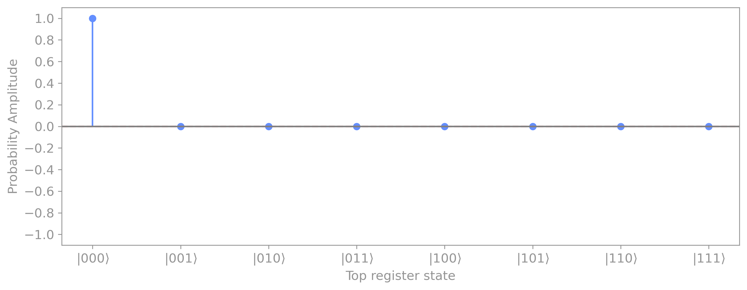
0. We start by initializing the top register in the all-zeros state and the bottom qubit in the minus state \(|\psi\rangle_0 = |0\rangle^{\otimes n} \otimes |-\rangle .\) This gives probability amplitudes for register \(x\) of:

\[\begin{split} \alpha_x^{(0)} = \begin{cases} 1, & \text{if } x = 0 \\ \\ 0, & \text{otherwise }. \end{cases} \end{split}\]

In the case of our 3-qubit example, at initialization we have state \(|000\rangle\) with amplitude of \(1\), and all other states with amplitudes of \(0,\) which we will display graphically for clarity:

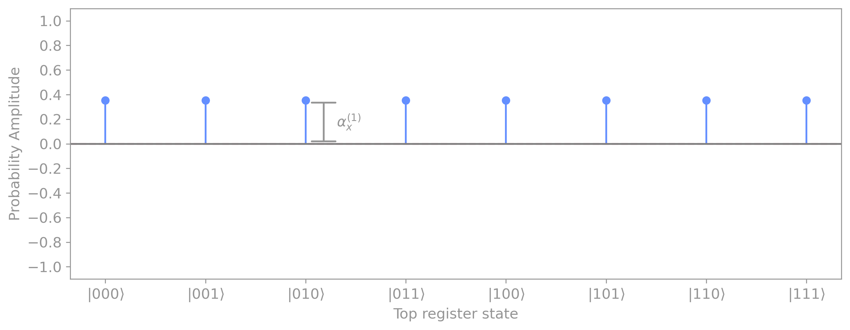
1. Next, we apply the \(\text{QHT}\) to register \(x\): \(|\psi\rangle_1 = \text{QHT}_n |0\rangle^{\otimes n} \otimes |-\rangle .\)

This places the top register in an equal superposition over all possible values of \(x,\) so all amplitudes take the same value:

\[\alpha_x^{(1)} = \frac{1}{\sqrt{N}}, \; \forall \; x.\]

For the 3-qubit example, this sets the probability amplitudes of all basis state to the same value of \(\alpha_x^{(1)} = 1 \big/\sqrt{8} \approx 0.3535:\)

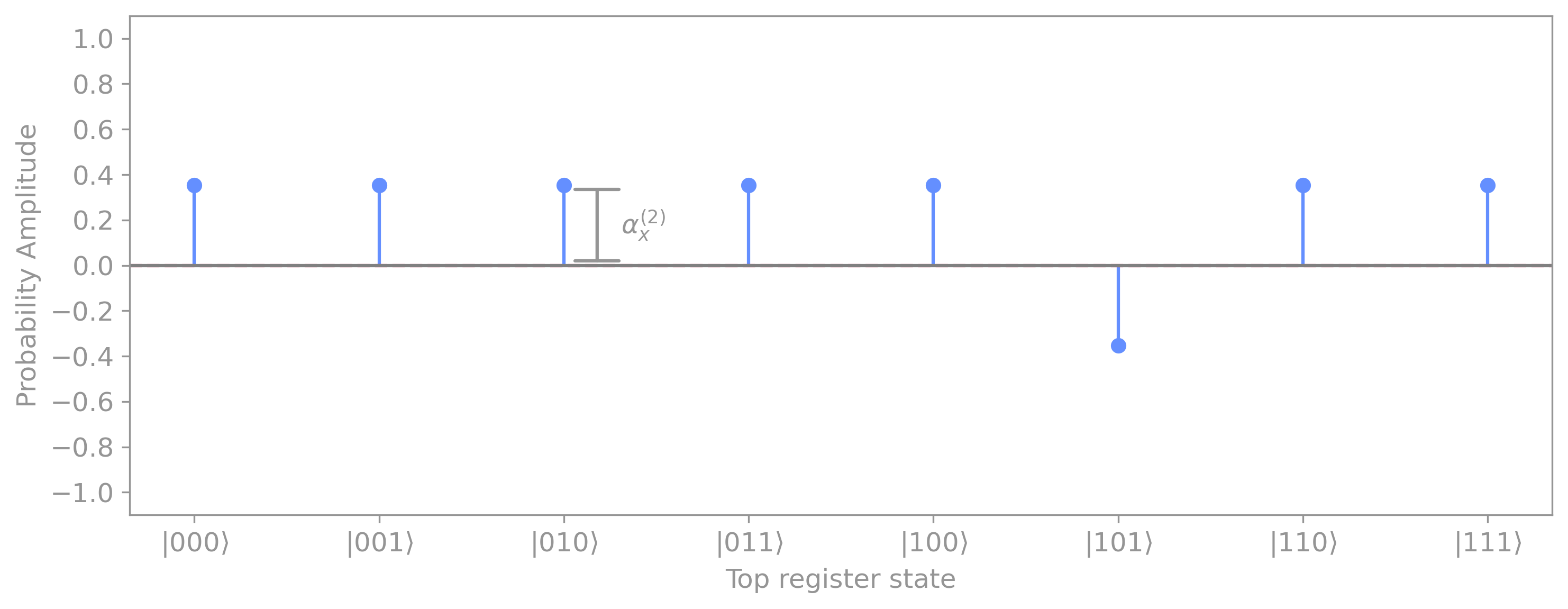
2. This is followed by evolving the state through the black box: \(|\psi\rangle_2 = U_f |\psi\rangle_1,\) which consists of performing quantum function evaluation over the superposition state. As we’ve seen before, for an arbitrary state \(|x\rangle,\) applying \(U_f\) (with the bottom qubit in state \(|-\rangle\)) produces a state of the form \((-1)^{f(x)} |x\rangle.\) Here we can note that, only the marked element \(m\) (for which \(f(x) = 1\)) its amplitude sees a sign inversion: \((-1)^{1} = -1.\) For all other states, we have \(f(x) = 0,\) so their amplitudes remain unchanged: \((-1)^{0} = 1.\)

\[\begin{split} \alpha_x^{(2)} = \begin{cases} \phantom{-} \frac{1}{\sqrt{N}}, & \text{if } x \neq m \\ \\ -\frac{1}{\sqrt{N}}, & \text{if } x = m . \end{cases} \end{split}\]

For our example, we have \(|101\rangle\) as our marked element, so this basis state will experience a change in sign:

3. We then perform amplitude amplification by evolving the state through the diffusion operator \(V.\) The way the amplitudes is amplified is by flipping all amplitudes about the mean value \(\mu\), which is given by the sum of all amplitudes divided by the number of elements:

\[ \mu^{(2)} = \frac{1}{N} \sum_{i = 0}^{N-1} \alpha_i^{(2)}. \]

Since at this point we have \((N - 1)\) elements with amplitude of \(\alpha_{i \neq m}^{(2)} = 1 \big / \sqrt{N}\) and \(1\) marked element with probability of \(\alpha_{i = m} = -1 \big / \sqrt{N},\) we can simplify the expression above as:

\[\begin{split} \begin{aligned} \mu^{(2)} &= \frac{1}{N} \left((N - 1)\frac{1}{\sqrt{N}} - \frac{1}{\sqrt{N}} \right) \\ \\ \mu^{(2)} &= \frac{1}{\sqrt{N}}\frac{N-2}{N}, \end{aligned} \end{split}\]

which for our example results in a mean value of:

\[ \mu^{(2)} = \frac{1}{\sqrt{8}}\frac{8-2}{8} \approx 0.265 .\]

To understand how the inversion about the mean works, it is helpful to show the relative distances between each probability amplitude to the mean (dotted line) given by \(\alpha_x^{(2)} - \mu^{(2)}:\)

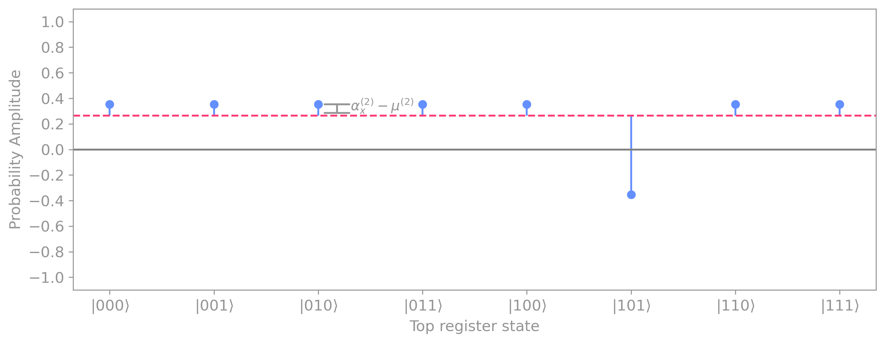
So after applying the diffuser there is a “reflection”, which flips the probability amplitudes with respect to the dotted line. The distance with respect to the mean is still the same, just in the opposite direction:

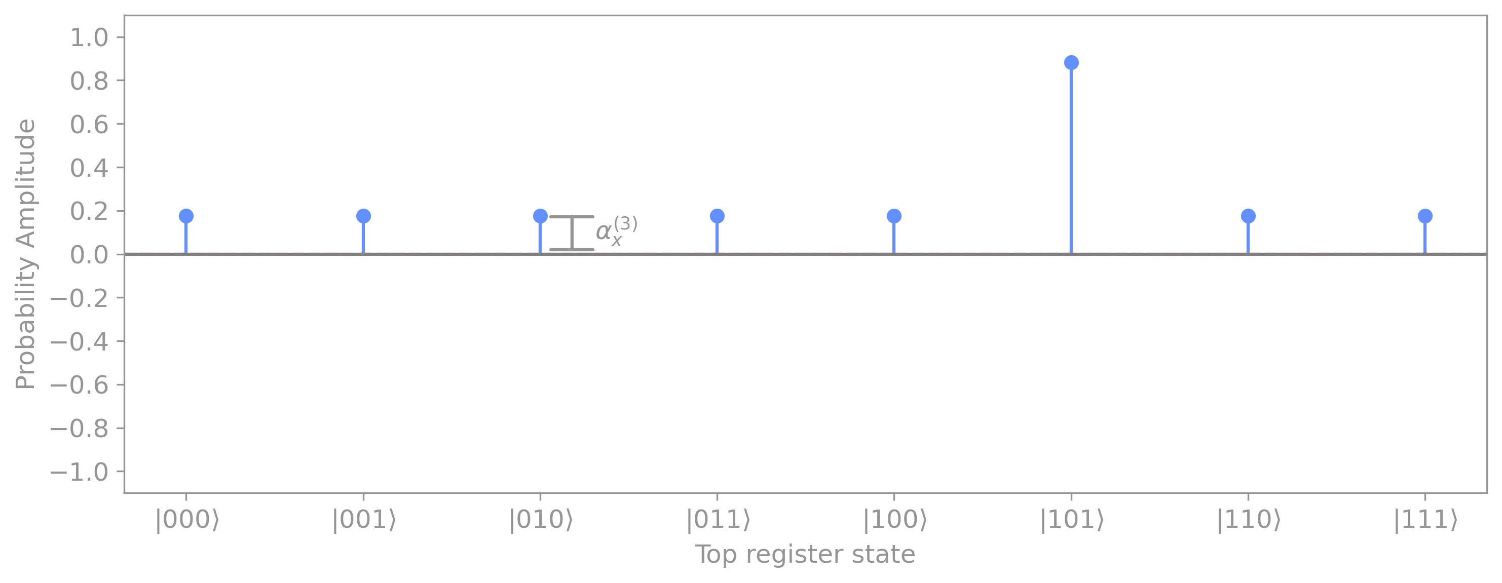
We can then calculate the new probability amplitudes \(\alpha_x^{(3)}\) after the diffuser, by subtracting this distance (\(\alpha_x^{(2)} - \mu^{(2)}\)) from the mean:

\[\begin{split} \begin{aligned} \alpha_x^{(3)} &= \mu^{(2)} - \left(\alpha_x^{(2)} - \mu^{(2)} \right) \\ \\ \alpha_x^{(3)} &= 2\mu^{(2)} - \alpha_x^{(2)} . \end{aligned} \end{split}\]

Replacing \(\mu^{(2)}\) and \(\alpha_x^{(2)}\) in the expression above, we can calculate the new probability amplitudes as:

\[\begin{split} \alpha_x^{(3)} = \begin{cases} \frac{1}{\sqrt{N}}\frac{N-4}{N}, & \text{if } x \neq m \\ \\ \frac{1}{\sqrt{N}}\frac{3N-4}{N}, & \text{if } x = m . \end{cases} \end{split}\]

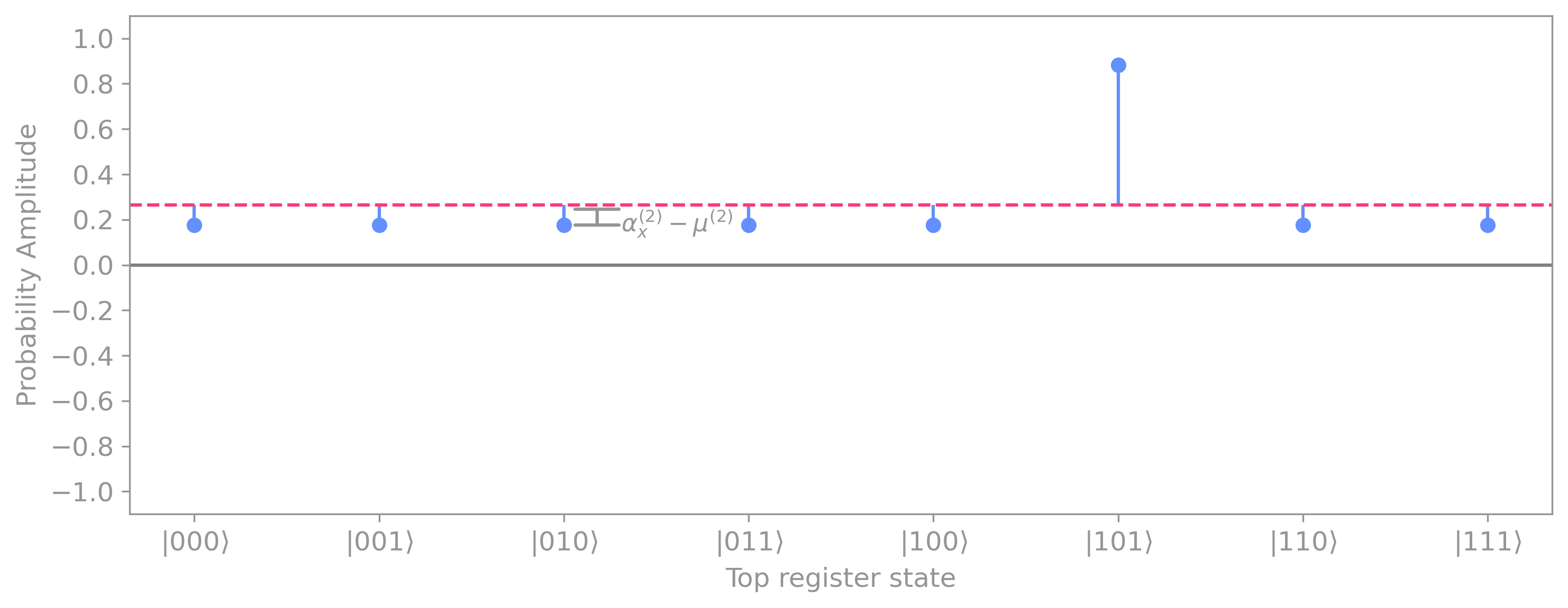
Since for 2 or more qubits we have: \(N \geq 4,\) the result above shows that applying \(V\) causes the probability amplitude of the marked element to increase in magnitude. This is evident in our example, where the new amplitude of the marked element is now clearly larger than that of the rest of the elements:

Specifically, we get:

\[\begin{split} \alpha_x^{(3)} = \begin{cases} \frac{1}{\sqrt{8}}\frac{8-4}{8} \approx 0.177, & \text{if } x \neq 101 \\ \\ \frac{1}{\sqrt{8}}\frac{3 \cdot 8 - 4}{8} \approx 0.884, & \text{if } x = 101 . \end{cases} \end{split}\]

This means that, if we were to perform a measurement right after applying \(V,\) we will find out marked element \(m = 101\) with probability:

\[ \mathbb{P}_{x = 101} \approx \left | 0.884 \right |^2 \approx 0.78 .\]

4. Surprisingly, we can do even better. If instead of measuring right away, we instead apply \(U_f\) again, the sign of the marked element will be flipped once again:

\[\begin{split} \alpha_x^{(4)} = \begin{cases} \phantom{-}\frac{1}{\sqrt{N}}\frac{N-4}{N}, & \text{if } x \neq m \\ \\ -\frac{1}{\sqrt{N}}\frac{3N-4}{N}, & \text{if } x = m . \end{cases} \end{split}\]

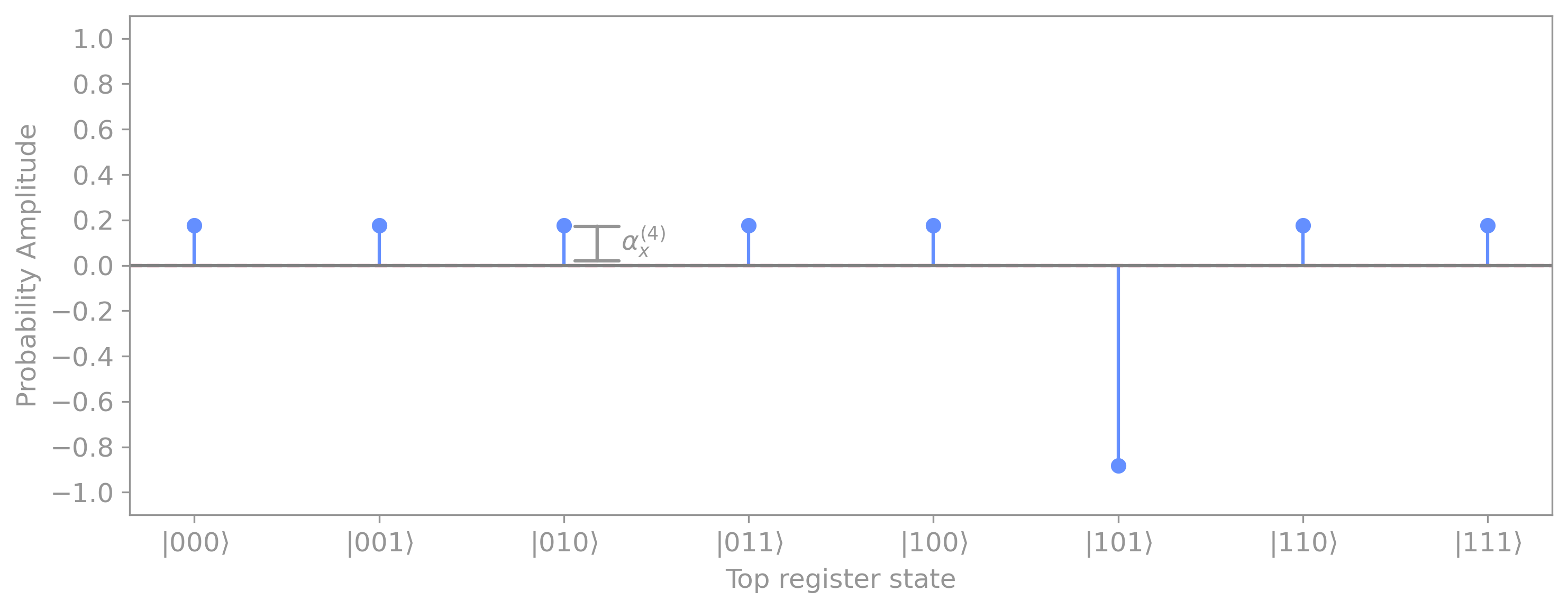
5. If we now recompute the mean:

\[ \mu^{(4)} = \frac{1}{N} \sum_{i = 0}^{N-1} \alpha_i^{(4)}, \]

and find the new probability amplitudes after reflecting about the mean by applying \(V\) again, results in:

\[ \alpha_x^{(5)} = 2\mu^{(4)} - \alpha_x^{(4)} .\]

Replacing the new average value \(\mu^{(4)}\) and the probability amplitudes \(\alpha_x^{(4)}\) for marked and unmarked elements give us:

\[\begin{split} \alpha_x^{(5)} = \begin{cases} \frac{1}{\sqrt{N}}\frac{N^2-12N+16}{N}, & \text{if } x \neq m \\ \\ \frac{1}{\sqrt{N}}\frac{5N^2-20N+16}{N}, & \text{if } x = m . \end{cases} \end{split}\]

For the case of \(N \geq 8\) (like in our example), the magnitude of the probability amplitude of the marked element increases even further:

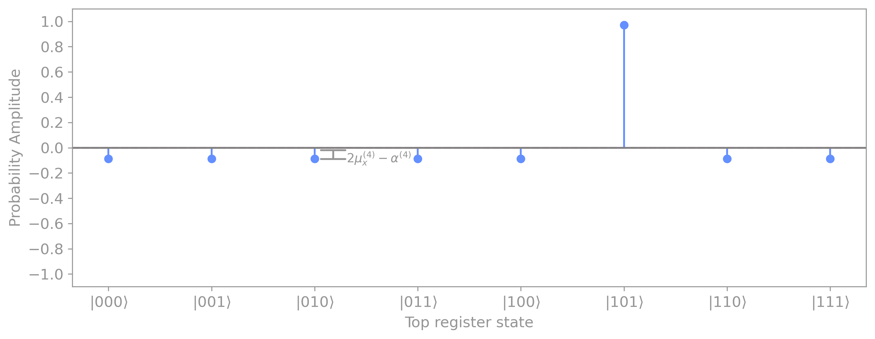
Specifically, we get:

\[\begin{split} \alpha_x^{(5)} = \begin{cases} \frac{1}{\sqrt{8}}\frac{8^2-12 \cdot 8 +16}{8} \approx -0.088, & \text{if } x \neq m \\ \\ \frac{1}{\sqrt{8}}\frac{5 \cdot 8^2-20 \cdot 8 + 16}{8} \approx 0.972, & \text{if } x = m , \end{cases} \end{split}\]

which results in a probability of measuring the marked element of:

\[ \mathbb{P}_{x = 101} \approx \left | 0.972 \right |^2 \approx 0.945 .\]

So after two applications of the oracle \(U_f\) and the diffuser \(V,\) we have managed to increase the probability of measuring the marked element from \(12.5 \%\) all the way up to \(94.5 \%.\)

Unfortunately, adding one more application of \(U_f\) and \(V\) actually decreases our chances of measuring the marked element. This occurs because the success probability follows a cyclical behavior rather than increasing monotonically. To understand why this is the case, and to determine the optimal number of iterations for a given number of elements, we must analyze Grover’s algorithm from a geometric perspective. Before doing so, however, let’s first examine how to construct the circuit that implements Grover’s diffusion operator \(V.\)

2.1.1 Grover’s Diffusion/Amplification Operator

As mentioned in the previous section, the role of Grover’s diffusion operator \(V\) is to reflect all probability amplitudes about their mean value. In this section, we will discuss how to construct the circuit that implements this unitary operation.

Given an arbitrary state at some circuit step \(t:\)

\[ |\psi\rangle_t = \sum \alpha_x^{(t)} |x\rangle, \]

the evolved state after applying \(V\) to \(|\psi\rangle_t\) is:

\[ |\psi\rangle_{t+1} = \sum \alpha_x^{(t+1)} |x\rangle. \]

where, as shown before, the updated probability amplitudes are given by:

\[ \alpha_x^{(t+1)} = 2 \mu^{(t)} - \alpha_x^{(t)} .\]

Again, here \(\mu^{(t)}\) is the amplitude mean at step \(t,\) expressed as:

\[ \mu^{(t)} = \frac{1}{N} \sum_{i=0}^{N -1} \alpha_i^{(t)} .\]

Our job is to find a unitary matrix \(V\) that performs the following transformation \(|\psi\rangle_{t+1} = V |\psi\rangle_{t},\) which written in vector form is:

\[\begin{split} \begin{aligned} \begin{bmatrix} \alpha_0 \\ \alpha_1 \\ \vdots \\ \alpha_{N-1} \end{bmatrix}^{(t+1)} &= \underbrace{\begin{bmatrix} * & * & \dots & * \\ * & * & \dots & * \\ \vdots & \vdots & \ddots & \vdots \\ * & * & \dots & * \end{bmatrix}}_V \begin{bmatrix} \alpha_0 \\ \alpha_1 \\ \vdots \\ \alpha_{N-1} \end{bmatrix}^{(t)} . \end{aligned} \end{split}\]

To do so, we can start by taking the statevector at step \(t+1,\) and replace every entry with the probability amplitude equation for \(\alpha_x^{(t+1)}\) evaluated at each value of \(x\):

\[\begin{split} \begin{aligned} \begin{bmatrix} \alpha_0 \\ \alpha_1 \\ \vdots \\ \alpha_{N-1} \end{bmatrix}^{(t+1)} &= \begin{bmatrix} 2 \mu - \alpha_0 \\ 2 \mu - \alpha_1 \\ \vdots \\ 2 \mu - \alpha_{N-1} \end{bmatrix}^{(t)} \\ \\ \begin{bmatrix} \alpha_0 \\ \alpha_1 \\ \vdots \\ \alpha_{N-1} \end{bmatrix}^{(t+1)} &= 2 \, \begin{bmatrix} \mu \\ \mu \\ \vdots \\ \mu \end{bmatrix}^{(t)} - \begin{bmatrix} \alpha_0 \\ \alpha_1 \\ \vdots \\ \alpha_{N-1} \end{bmatrix}^{(t)} . \end{aligned} \end{split}\]

Here, we can make use of the fact that the average \(\mu\) of any vector \(|\psi\rangle\) can be computed by performing the inner product between the vector itself and the all-ones vector \(|1\rangle^{\otimes n}\), and dividing by the total number of elements:

\[\begin{split} \begin{aligned} \mu &= \frac{1}{N} \langle 1|^{\otimes n} |\psi\rangle \\ \\ \mu &= \frac{1}{N} \begin{bmatrix} 1 & 1 & \dots & 1 \end{bmatrix} \begin{bmatrix} \alpha_0 \\ \alpha_1 \\ \vdots \\ \alpha_{N-1} \end{bmatrix} . \end{aligned} \end{split}\]

Replacing \(\mu\) in the expression above:

\[\begin{split} \begin{aligned} \begin{bmatrix} \alpha_0 \\ \alpha_1 \\ \vdots \\ \alpha_{N-1} \end{bmatrix}^{(t+1)} &= \frac{2}{N} \begin{bmatrix} 1 & 1 & \dots & 1 \\ 1 & 1 & \dots & 1 \\ \vdots & \vdots & \ddots & \vdots \\ 1 & 1 & \dots & 1 \end{bmatrix} \begin{bmatrix} \alpha_0 \\ \alpha_1 \\ \vdots \\ \alpha_{N-1} \end{bmatrix}^{(t)} - \begin{bmatrix} \alpha_0 \\ \alpha_1 \\ \vdots \\ \alpha_{N-1} \end{bmatrix}^{(t)} . \end{aligned} \end{split}\]

And finally, factorizing the vector at step \(t\) gives us:

\[\begin{split} \begin{aligned} \begin{bmatrix} \alpha_0 \\ \alpha_1 \\ \vdots \\ \alpha_{N-1} \end{bmatrix}^{(t+1)} &= \underbrace{\left(\frac{2}{N} \begin{bmatrix} 1 & 1 & \dots & 1 \\ 1 & 1 & \dots & 1 \\ \vdots & \vdots & \ddots & \vdots \\ 1 & 1 & \dots & 1 \end{bmatrix} - \begin{bmatrix} 1 & 0 & \dots & 0 \\ 0 & 1 & \dots & 0 \\ \vdots & \vdots & \ddots & \vdots \\ 0 & 0 & \dots & 1 \end{bmatrix} \right)}_V \begin{bmatrix} \alpha_0 \\ \alpha_1 \\ \vdots \\ \alpha_{N-1} \end{bmatrix}^{(t)}. \end{aligned} \end{split}\]

As seen, \(V\) can be written as the difference of two matrices. A convenient way to write the first matrix is as the outer product of the equal superposition state:

\[\begin{split} |s\rangle = \frac{1}{\sqrt{N}} \sum_{x = 0}^{N-1} |x\rangle = \frac{1}{\sqrt{N}} \begin{bmatrix} 1 \\ 1 \\ \vdots \\ 1 \end{bmatrix} \end{split}\]

Taking the outer product of this state with itself:

\[\begin{split} \begin{aligned} |s\rangle \langle s| &= \frac{1}{\sqrt{N}} \begin{bmatrix} 1 & 1 & \dots & 1 \end{bmatrix} \frac{1}{\sqrt{N}} \begin{bmatrix} 1 \\ 1 \\ \vdots \\ 1 \end{bmatrix} \\ \\ |s\rangle \langle s| &= \frac{1}{N} \begin{bmatrix} 1 & 1 & \dots & 1 \\ 1 & 1 & \dots & 1 \\ \vdots & \vdots & \ddots & \vdots \\ 1 & 1 & \dots & 1\end{bmatrix} . \end{aligned} \end{split}\]

and the second matrix is simply the identity matrix:

\[\begin{split} I = \begin{bmatrix} 1 & 0 & \dots & 0 \\ 0 & 1 & \dots & 0 \\ \vdots & \vdots & \ddots & \vdots \\ 0 & 0 & \dots & 1 \end{bmatrix} . \end{split}\]

Therefore, we can write \(V\) as:

\[ \boxed{V = 2|s\rangle \langle s| - I }\]

This is a nice definition, and one that we will use later. However, it doesn’t really tell us much about how to construct the circuit that generates \(V.\) For this, we need to take advantage of two important facts:

1. The equal-superposition state \(|s\rangle\) is generated by applying the \(\text{QHT}\) to the all-zeros state:

\[ |s\rangle = \text{QHT}_n |0\rangle^{\otimes n}. \]

So we can write:

\[\begin{split} \begin{aligned} |s\rangle \langle s| &= \text{QHT}|0\rangle \big(\text{QHT}|0\rangle \big)^{\dagger} \\ \\ |s\rangle \langle s| &= \text{QHT}\big(|0\rangle \langle 0|\big)\text{QHT}, \end{aligned} \end{split}\]

where we have omitted the \(n\) sub/superscripts for convenience and make use of the fact that \(\text{QHT}^{\dagger} = \text{QHT}.\)

2. We can sandwich the identity operator between two \(\text{QHT}\) operators and still get the identity:

\[ I = \text{QHT} \big(\, I \,\big) \text{QHT}. \]

Replacing these two in the expression for \(V\) yields:

\[\begin{split} \begin{aligned} V &= 2|s\rangle \langle s| - I \\ \\ V &= 2 \, \text{QHT}\big(|0\rangle \langle 0|\big)\text{QHT} - \text{QHT} \big(\, I \,\big) \text{QHT} \\ \\ V &= \text{QHT}\big(2 |0\rangle \langle 0| - I \big) \text{QHT}. \end{aligned} \end{split}\]

This doesn’t seem to have gotten us any closer since we still have \(V\) as the difference of two matrices. However, if we explicitly write this in matrix form:

\[\begin{split} \begin{aligned} 2 |0\rangle \langle 0| - I &= \begin{bmatrix}2 & 0 & \dots & 0 \\ 0 & 0 & \dots & 0 \\ \vdots & \vdots & \ddots & \vdots \\ 0 & 0 & \dots & 0 \end{bmatrix} - \begin{bmatrix} 1 & 0 & \dots & 0 \\ 0 & 1 & \dots & 0 \\ \vdots & \vdots & \ddots & \vdots \\ 0 & 0 & \dots & 1 \end{bmatrix} \\ \\ 2 |0\rangle \langle 0| - I &= \begin{bmatrix}1 & 0 & \dots & 0 \\ 0 & -1 & \dots & 0 \\ \vdots & \vdots & \ddots & \vdots \\ 0 & 0 & \dots & -1 \end{bmatrix} \\ \\ 2 |0\rangle \langle 0| - I &= -1 \, \begin{bmatrix}-1 & 0 & \dots & 0 \\ 0 & 1 & \dots & 0 \\ \vdots & \vdots & \ddots & \vdots \\ 0 & 0 & \dots & 1 \end{bmatrix} . \end{aligned} \end{split}\]

The result is a diagonal matrix where the first element is \(-1,\) and the remaining diagonal terms are \(1.\) The matrix is also pre-multiplied by a global phase of \(-1,\) but as we’ve discussed before, global phases do not have an effect on the final measurement results of a circuit, so we can ignore it.

A matrix of this type basically adds a phase of \(-1\) to the all-zeros state \(|0\rangle^{\otimes n},\) and leaves all other states alone. Recall from the section on controlled gates that corresponds to a multi-controlled \(Z\) gate that gets activated when all qubits are \(|0\rangle.\) We can then express the diffusion operator as:

\[ V = \text{QHT} \; M\overline{C}Z \; \text{QHT}, \]

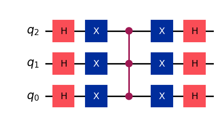
where \(M\overline{C}Z\) corresponds to the aforementioned multi-controlled \(Z,\) which can be implemented using a conventional \(MCZ\) gate, sandwiched in between \(X\) gates on every qubit:

\[ V = \text{QHT} \; X^{\otimes n} \; MCZ \; X^{\otimes n} \; \text{QHT}, \]

The qiskit code below generates a diffusion operator for an arbitrary number of qubits \(n\).

from qiskit.circuit.library import ZGate

def diffuser(n):
    
    mcz = ZGate().control(n-1)
    
    qc_v = QuantumCircuit(n, name=' $V$ (Diffuser)')
    qc_v.h(range(n))
    qc_v.x(range(n))
    qc_v.append(mcz,range(n))
    qc_v.x(range(n))
    qc_v.h(range(n))
    
    return qc_v

n = 3 # number of qubits

qc_diff = diffuser(3)
qc_diff.draw()

Now we have all the ingredients to implement Grover’s algorithm. What is left, is to find what is the number of repetitions \(\kappa\) needed to maximize the probability of finding the marked element \(m.\)

2.2 Number of Iterations

In the section above, we found that the probability amplitudes after each application of the oracle \(U_f\) and the diffuser \(V\) are updated as:

\[ \alpha_x^{(t+1)} = 2\mu^{(t)} - \alpha_x^{(t)} \quad \forall \; x,\]

where \(\mu^{(t)}\) is the mean of the probability amplitudes given by:

\[ \mu^{(t)} = \frac{1}{N}\big[ (N-1) \, \alpha_{x \neq m}^{(t)} + \alpha_{x = m}^{(t)} \big] .\]

A way of finding the required number of applications \(\kappa\) to measure the marked element \(m\) with high probability, is to iterate over the recursive expression above until the probability amplitude of the marked element \(\alpha_{x=m}\) stops increasing.

Let’s write a python function that accomplishes this:

def find_κ(N):
    
    κ = 0                 # Number of iteration
    α_max = 1/np.sqrt(N)  # variable to track max prob amp of marked state 
    

    # Define initial prob amplitudes of marked and unmarked elements
    α_marked = α_max
    α_unmarked = α_max
    
    # Iterate until new prob amplitude of marked element stops increasing in magnitude
    while True:
        
        # Flip amplitude of marked element
        α_marked = -α_marked
        
        # Compute mean
        μ = ((N-1)*α_unmarked + α_marked)/N
        
        # Recompute amplitudes
        α_marked = 2*μ - α_marked
        α_unmarked = 2*μ - α_unmarked
        
        if abs(α_marked) < α_max:
            break
        else:
            α_max = abs(α_marked)
            κ += 1
            
    return κ

n = 5
N = 2**n
κ = find_κ(N)

print(f'Number of repetions needed to find 1 marked element among {N} elements is κ = {κ}.')

Number of repetions needed to find 1 marked element among 32 elements is κ = 4.

The method above works well. However, there is a more elegant way to analyze Grover’s algorithm that allows us to find a close-form expression for \(\kappa.\)

Let’s start by noting that the equal superposition over all basis states \(|s\rangle\) can be separated into two orthogonal states; one given by the marked state \(|m\rangle,\) and the other by all remaining basis states:

\[\begin{split} \begin{aligned} |s\rangle &= \sqrt{\frac{1}{N}} \sum_{x=0}^{N-1} |x\rangle \\ \\ |s\rangle &= \sqrt{\frac{N-1}{N}} \sum_{x\neq 0} |x\rangle + \sqrt{\frac{1}{N}} |m\rangle \\ \\ |s\rangle &= \sqrt{\frac{N-1}{N}} |m^\perp \rangle + \sqrt{\frac{1}{N}} |m\rangle \end{aligned} \end{split}\]

So, for example, if we have the marked element \(m = 101:\)

\[\begin{split} \begin{aligned} |m\rangle &= |101\rangle \\ \\ |m^\perp \rangle &= |000\rangle + |001\rangle + |010\rangle + |011\rangle + |100\rangle + |110\rangle + |111\rangle. \end{aligned} \end{split}\]

It is not hard to see that these two states are orthogonal because \(\langle m | m^\perp \rangle = 0.\) As such, we can graphically represent these in an abstract \(xy\)-plane plane with \(|m\rangle\) as the \(y\) axis, and \(|m^\perp \rangle\) as the \(x\) axis. We can then draw the state \(|s\rangle\) as a vector within this plane with coordinates: \(\left(\sqrt{\frac{N-1}{N}}, \sqrt{\frac{1}{N}}\right).\)

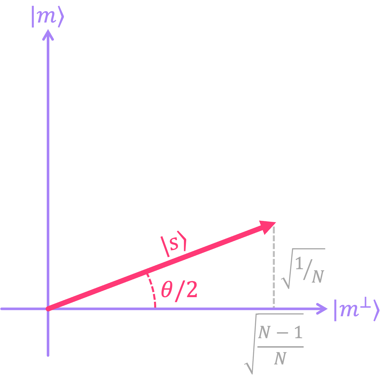
From this image, we can also see that we can express \(|s\rangle\) in terms of the angle \(\theta\) as:

\[ |s\rangle = \cos\left( \frac{\theta}{2} \right) |m^\perp \rangle + \sin \left(\frac{\theta}{2} \right) |m \rangle ,\]

where the angle is given by:

\[\begin{split} \begin{aligned} \sin \left(\frac{\theta}{2} \right) &= \frac{1}{\sqrt{N}} \\ \\ \theta &= 2 \sin^{-1}\left(\frac{1}{\sqrt{N}} \right). \end{aligned} \end{split}\]

With this picture in mind, we can then analyze how a statevector evolves through Grover’s algorithm.

The first step, is to place the top input register in the equal superposition state \(|s\rangle\) and the auxiliary bottom qubit in state \(|-\rangle.\) However, we leave the bottom qubit out of this analysis since we know it is only used for the phase kickback effect and always remains unentangled.

We then apply \(U_f\) to our state, which flips the amplitude of the marked element \(|m\rangle\). In our diagram, this is equivalent to reflecting \(|s\rangle\) about the \(|m^\perp \rangle\) axis:

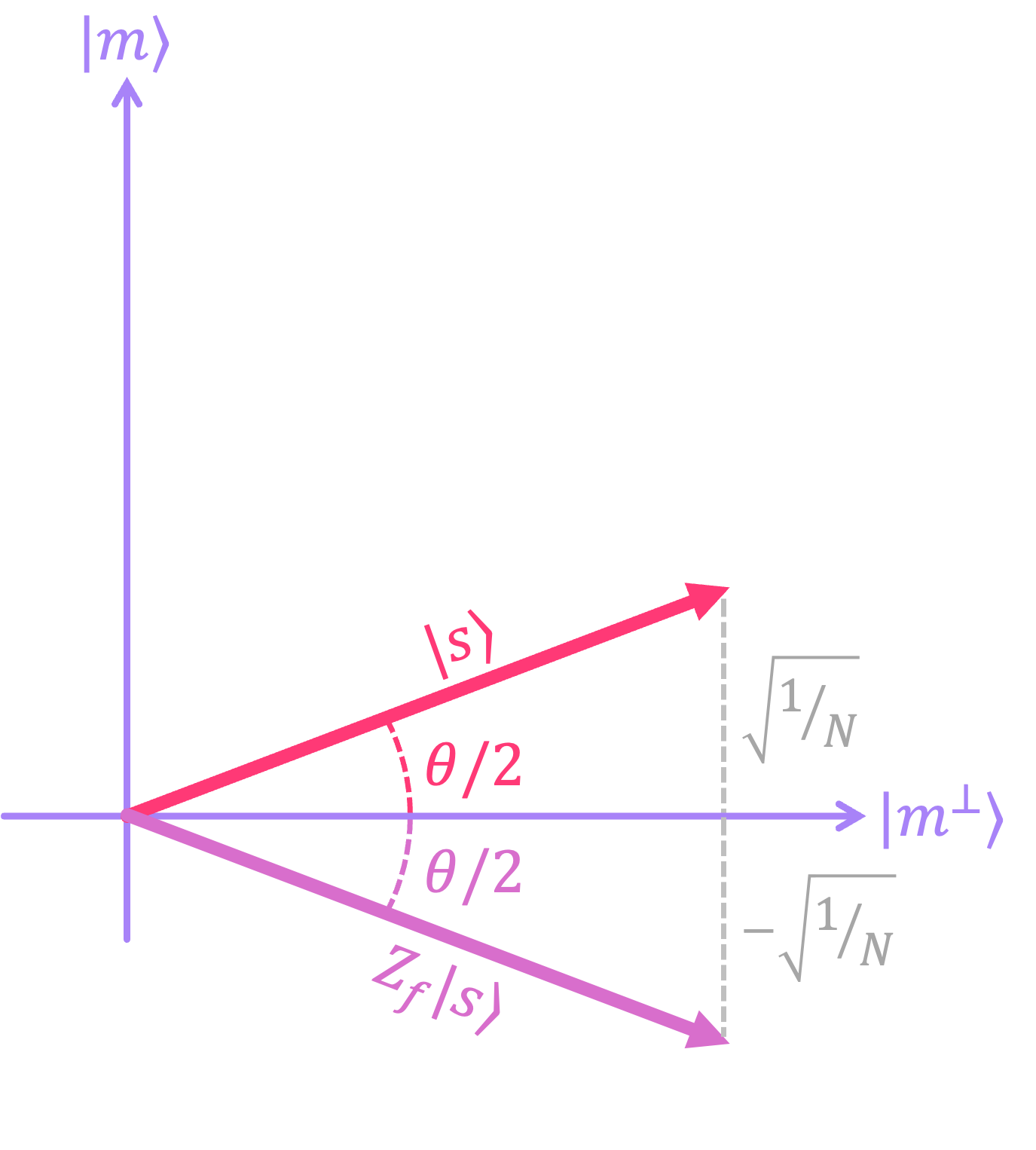
NOTE: In the diagram above, the state after applying \(U_f\) is written as \(Z_f |s\rangle\) because, as explained in the section on quantum oracles, a bit oracle like \(U_f\) is equivalent to the phase oracle \(Z_f\) when the bottom qubit is initialized in state \(|-\rangle.\)

The next step, is to apply \(V.\) It turns out that this operation corresponds to a reflection about \(|s\rangle\), so the resulting state is oriented at an angle of \(\theta\) with respect to the starting vector:

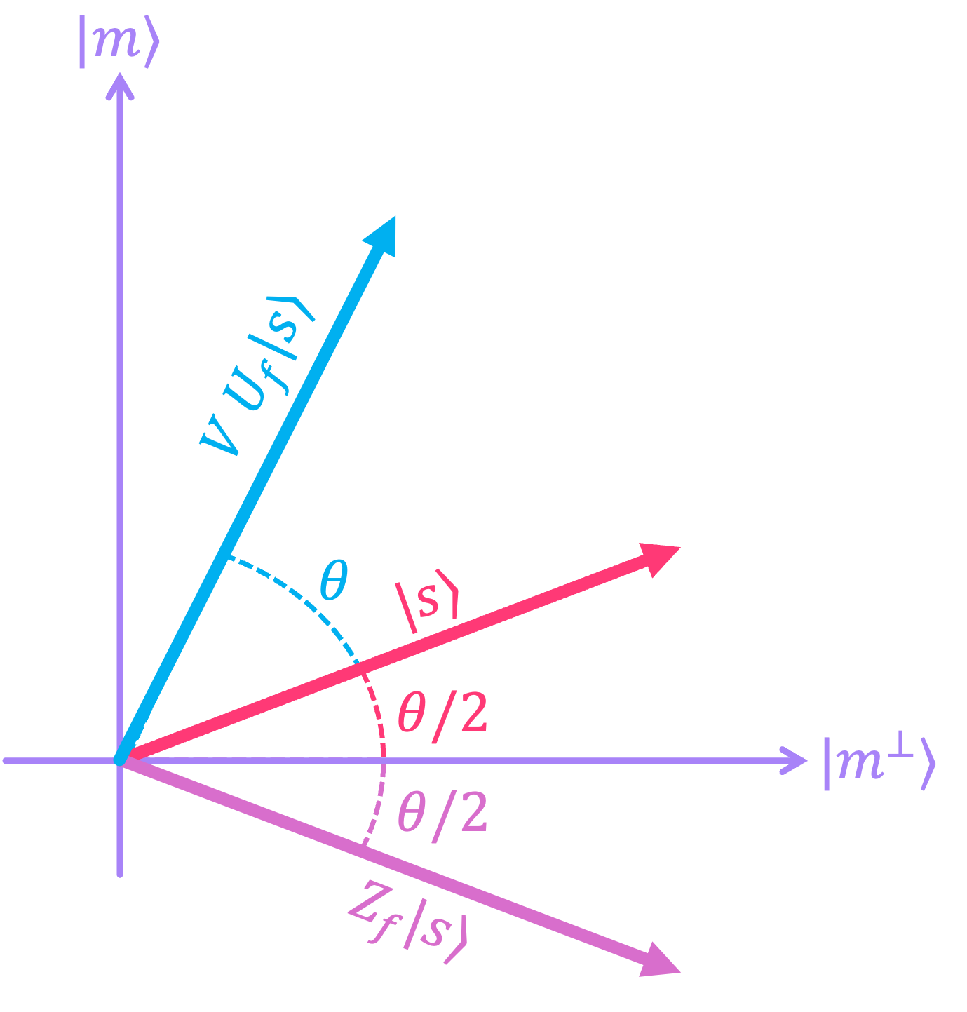
What’s more, Every application of \(\left(V U_f\right)\) is an additional rotation by \(\theta.\) So for two applications, (i.e., applying \((U_f V)^2\) to \(|s\rangle)\) the initial state is rotated by \(2\theta.\)

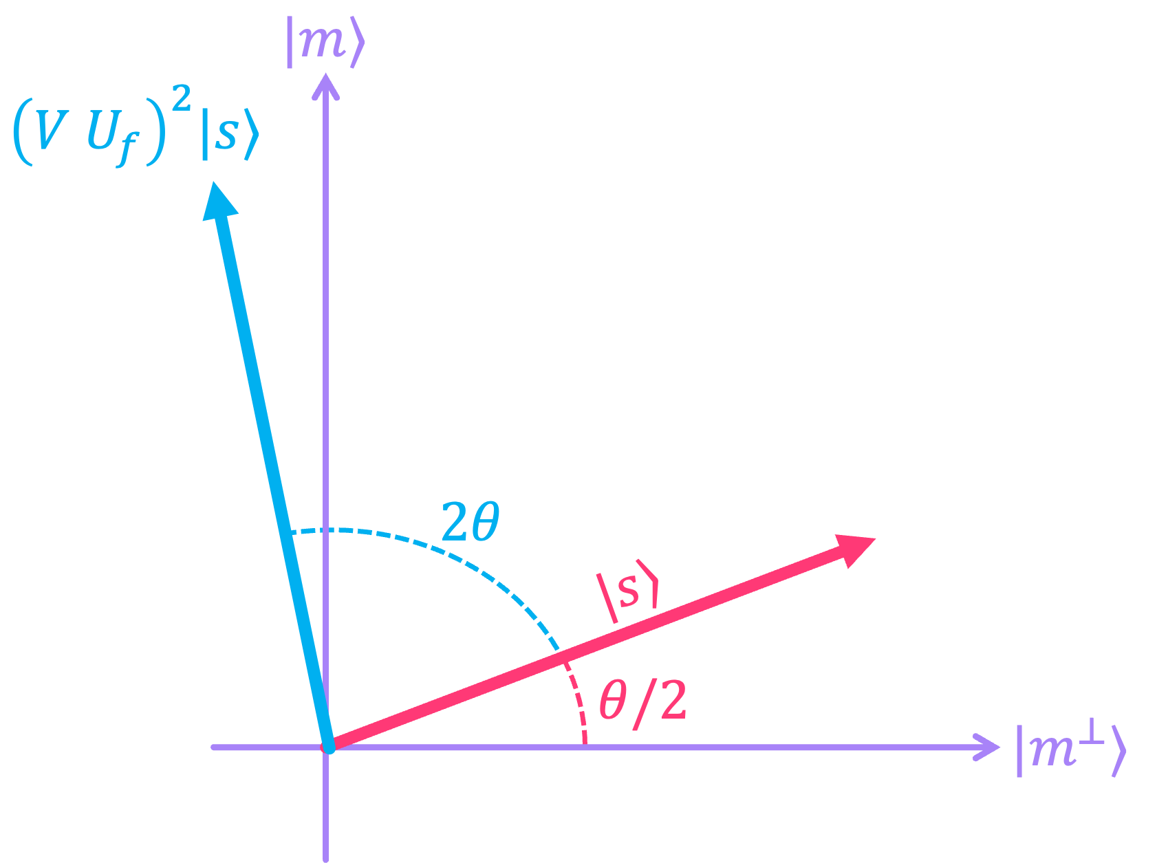
In general, the operation \((V U_f)^\kappa\) rotates the initial superposition state by \(\kappa \theta.\)

Recall that the goal of Grover’s algorithm is to get the vector \((V U_f )^\kappa|s\rangle\) as close as possible to the axis \(|m\rangle,\) which represents our marked element. This means that, what we want after \(\kappa\) applications of \(U_f\) and \(V\), is for the vector to point an angle of \(\pi/2.\) This requires meeting the following condition:

\[ \kappa \theta + \frac{\theta}{2} = \frac{\pi}{2} .\]

Solving for \(\kappa\) and replacing \(\theta:\)

\[\begin{split} \begin{aligned} \kappa &= \frac{\pi}{2\theta} - \frac{1}{2} \\ \\ \kappa &= \frac{\pi}{4\sin^{-1}\left(1 \big/\sqrt{N} \right)} - \frac{1}{2}. \end{aligned} \end{split}\]

Given that \(\kappa\) corresponds to a whole number of iterations, we actually need to find the closest integer:

\[ \boxed{\kappa = \left \lfloor \frac{\pi}{4\sin^{-1}\left(1 \big/\sqrt{N} \right)} - \frac{1}{2} \right \rceil} \]

We can write this expression in python, and show that this expression gives the same result as what we obtained using the recursive method above:

n = 5
N = 2**n
κ = round(np.pi/(4*np.arcsin(1/np.sqrt(N)))-1/2)

print(f'Number of repetions needed to find 1 marked element among {N} elements is κ = {κ}.')

Number of repetions needed to find 1 marked element among 32 elements is κ = 4.

As expected, if we take the expression above in the limit where \(N\) is large, we find that \(\kappa\) (which also represents the number of calls to \(U_f\)) grows proportional to \(\sqrt{N}.\)

With this, we are now ready to implement Grover’s algorithm to search for 1 marked element.

2.3 Python Implementation

First, let’s create a function that generates Grover’s quantum circuit for \(\kappa\) repetitions of \(U_f\) and \(V:\)

def grover_one_marked(n, κ):
    
    bb, m = Uf_one_marked(n)
    
    qc_g = QuantumCircuit(n+1,n)
    qc_g.x(0)
    qc_g.h(0)
    qc_g.barrier()
    qc_g.h(range(1,n+1))
    
    for _ in range(κ):
        qc_g.append(bb,range(n+1))
        qc_g.append(diffuser(n),range(1,n+1))

    qc_g.barrier()
    qc_g.measure(range(1,n+1),range(n))
    
    return qc_g, m

The function above uses the same black box function \(U_f\) that we implemented for the classical case, where the marked element \(m\) is selected at random. Let’s generate a circuit example and run it several times to verify that the most likely outcome is the marked element.

from qiskit import transpile
from qiskit.visualization import plot_distribution
from qiskit_aer import AerSimulator

n = 3                                             # Number of qubits
N = 2**n                                          # Number of elements
κ = round(np.pi/(4*np.arcsin(1/np.sqrt(N)))-1/2)  # Number of iterations

qc, m = grover_one_marked(n, κ)
qc.draw()

simulator = AerSimulator()

qc_t = transpile(qc, simulator)
job = simulator.run(qc_t, shots=2**13)
counts = job.result().get_counts()

print(f'Secret marked element: m = {m}')
plot_distribution(counts, title='Frequency of measuring each element')

Secret marked element: m = 010

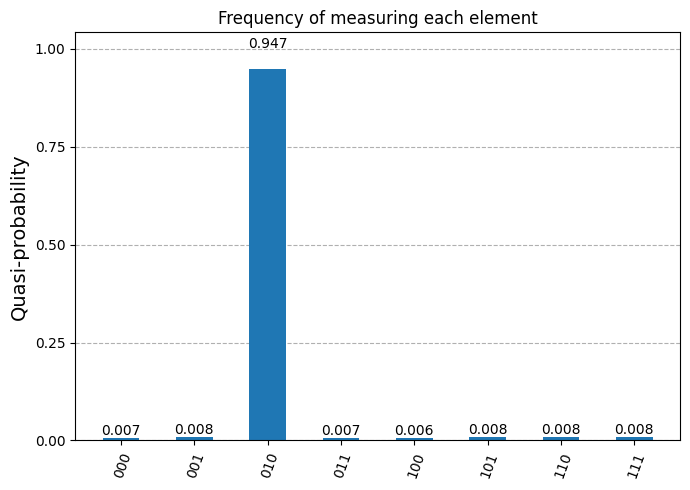
As seen, the marked element is always measured with high probability.

Now, a nice thing about Grover’s algorithm is that, even though there is a small probability of not measuring the marked element, we can always run the algorithm once, extract the output \(x_{out}\), and evaluate \(U_{f(x)}\) on this value to check if we were successful. If \(f(x_{out}) = 1,\) we know is \(x_{out}=m.\) If not, we can rerun the algorithm and check again. The image below shows a flow diagram of the steps required to successfully extract \(m\) using Grover’s algorithm.

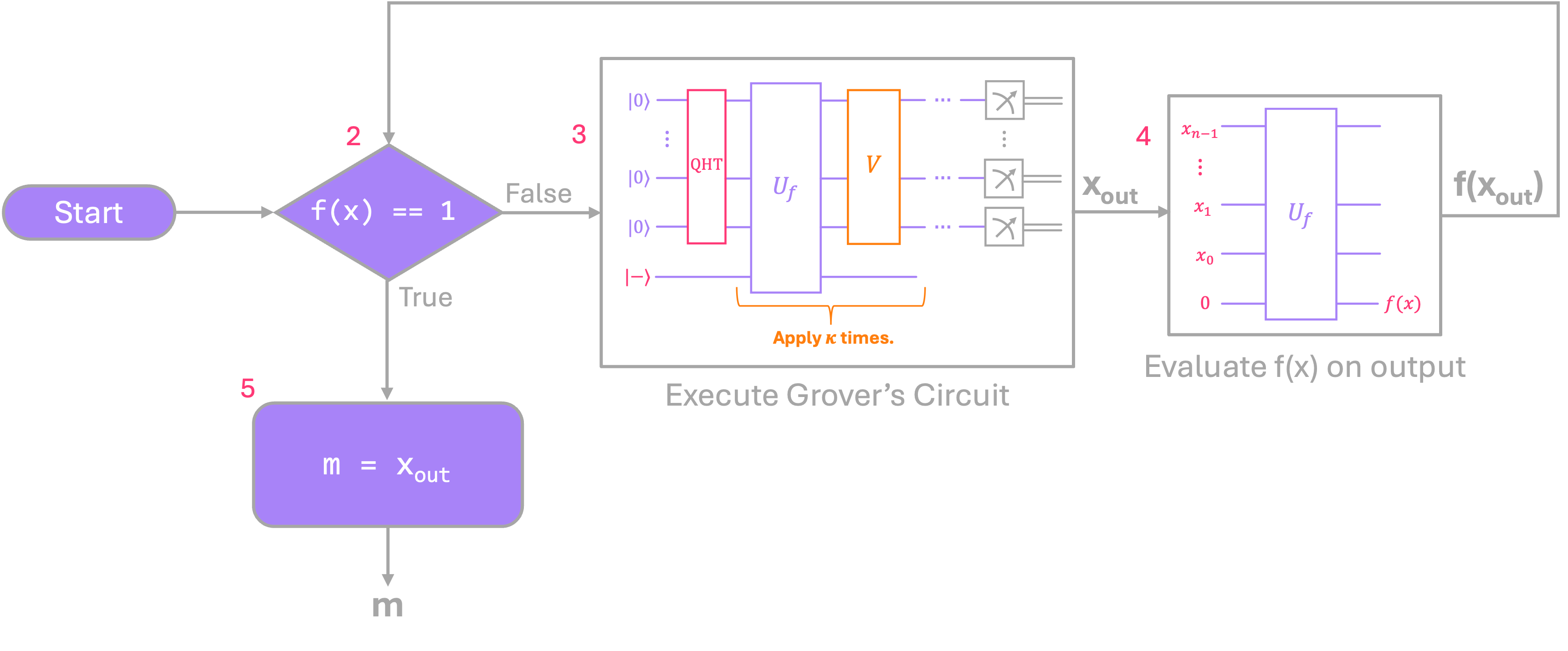
1. Start the algorithm by first computing the number of iterations needed κ.

2. Check if the output of Grover’s algorithm x_out is equal to 1.

3. If not, run Grover’s algorithm.

4. Evaluate the output of Grover’s circuit on f(x) and go back to step 2 to check if it evaluates to 1.

5. If f(x) == 1, then the output of Grover’s the circuit is the marked element m.

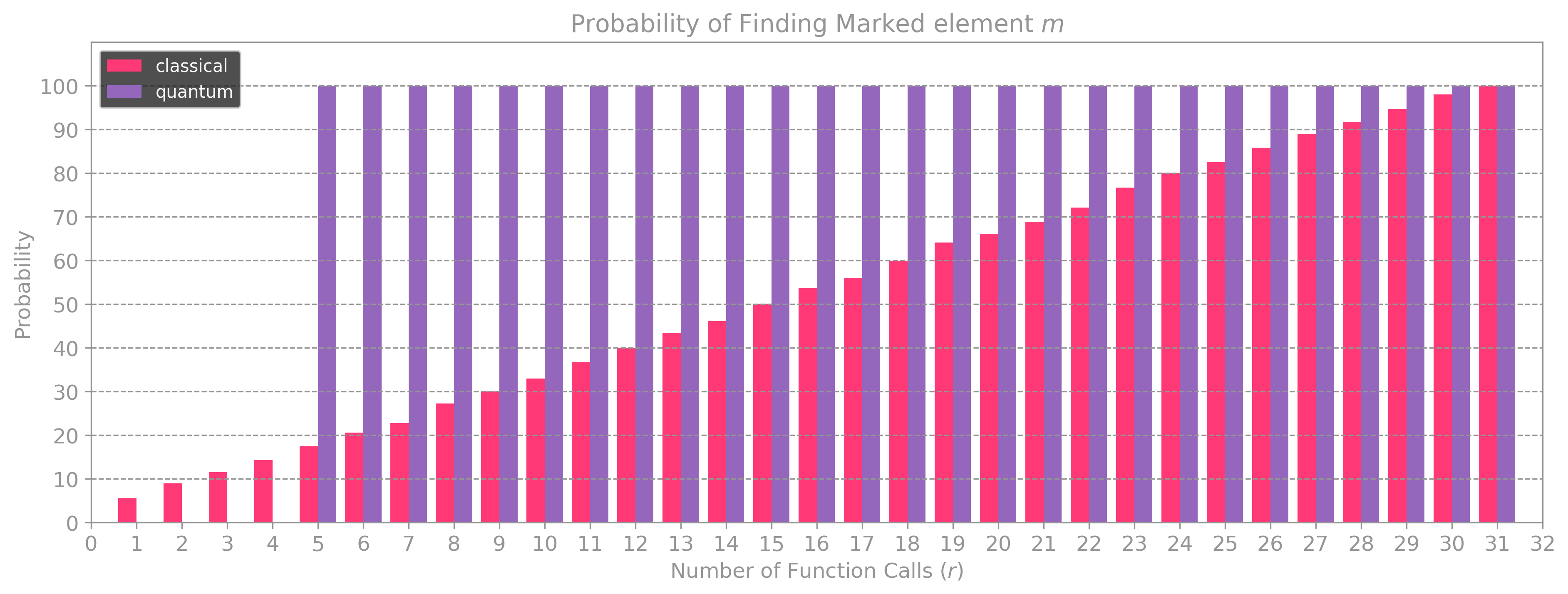
With this procedure, we will need a minimum of \(\kappa +1 \) evaluations of \(U_f\) to find \(m.\) The plot below shows a comparison between the probability of finding the marked element \(m\) for a given number of calls \(r\) to \(U_f\) when using classical queries vs. Grover’s algorithm. As seen, for \(N = 32\) elements, the probability of finding \(m\) using Grover’s algorithm is close to \(100 \%\) after \(\kappa + 1 = 5\) calls, which is quadratically better than the classical case, which requires going over all \(32\) elements.

3. Generalizing for M Marked Elements

All previous analysis was for the case where we need to find one marked element \(m\) among \(N\) total elements. But Grover’s algorithm generalizes for when there are \(M\) marked elements. The algorithm remains the same, but the number of iterations \(\kappa\) needs to be re-calculated.

The procedure to find \(\kappa\) identical to what we covered in section 2.2, where we start by defining the initial superposition statevector \(|s\rangle\) in terms of two orthogonal states:

\[\begin{split} \begin{aligned} |s\rangle &= \sqrt{\frac{N-M}{N}} \sum_{x \notin \Xi} |x\rangle + \sqrt{\frac{M}{N}} \sum_{m \in \Xi} |m\rangle \\ \\ |s\rangle &= \sqrt{\frac{N-M}{N}} |\xi^\perp \rangle + \sqrt{\frac{M}{N}} |\xi\rangle . \end{aligned} \end{split}\]

Here, \(\Xi\) is the set of \(M\) marked elements.

Let’s take for example the case of for \(N = 8\) total elements, and \(M = 2\) marked elements: \(\Xi = \{010, 110\}.\) We then have:

\[\begin{split} \begin{aligned} |\xi\rangle &= |010\rangle+|110\rangle \\ \\ |\xi^\perp \rangle &= |000\rangle + |001\rangle + |011\rangle + |100\rangle + |101\rangle + |111\rangle. \end{aligned} \end{split}\]

Since \(\langle\xi|\xi^\perp \rangle = 0,\) we express equal superposition state as:

\[|s\rangle = \cos\left(\frac{\theta}{2} \right) |\xi^\perp \rangle + \sin\left(\frac{\theta}{2} \right) |\xi\rangle .\]

This means that:

\[\begin{split} \begin{aligned} \sin \left(\frac{\theta}{2} \right) &= \sqrt{\frac{M}{N}} \\ \\ \theta &= 2 \sin^{-1}\left(\sqrt\frac{M}{N} \right), \end{aligned} \end{split}\]

which we can replace in the same equation we used before to find \(\kappa:\)

\[ \kappa = \left \lfloor \frac{\pi}{4\sin^{-1}\left(\sqrt{M \big/ N} \right)} - \frac{1}{2} \right \rceil. \]

Let’s now create an oracle \(U_f\) that generates some random \(M\) number of marked elements, and run Grover’s algorithm on it to find them.

def Uf_M_marked(n, M):
    N = 2**n
    
    if M >= N:
        M = N - 1
    
    m_int_lst = np.random.randint(N, size=M)
    m_lst = [np.binary_repr(m_int,n) for m_int in m_int_lst]
    qc_bb = QuantumCircuit(n+1, name=' $U_f$ (Oracle)')
    
    for m in m_lst:
        qc_bb.mcx(list(range(1,n+1)),0, ctrl_state=m)
    
    return qc_bb, m_lst

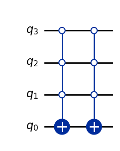
qc, m_lst = Uf_M_marked(3, 2)

print(f'marked elements: {m_lst}')
qc.draw()

marked elements: ['000', '000']

def grover_M_marked(n, M, κ):
    
    bb, m_lst = Uf_M_marked(n, M)
    
    qc_g = QuantumCircuit(n+1,n)
    qc_g.x(0)
    qc_g.h(0)
    qc_g.barrier()
    qc_g.h(range(1,n+1))
    
    for _ in range(κ):
        qc_g.append(bb,range(n+1))
        qc_g.append(diffuser(n),range(1,n+1))

    qc_g.barrier()
    qc_g.measure(range(1,n+1),range(n))
    
    return qc_g, m_lst

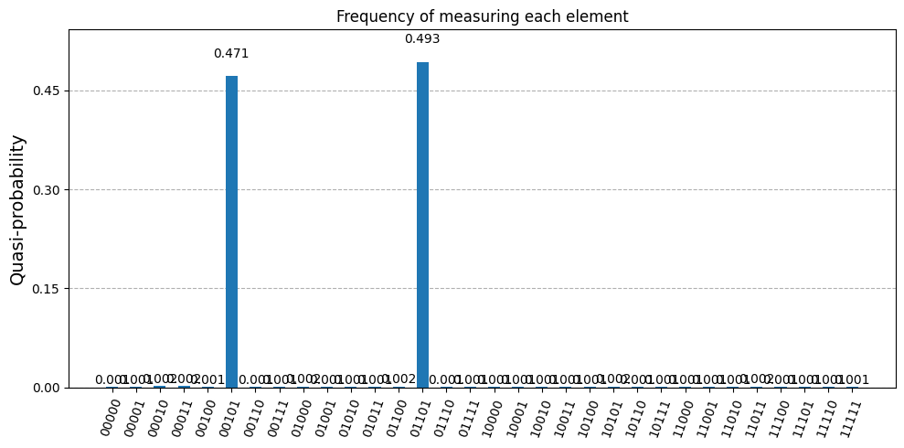
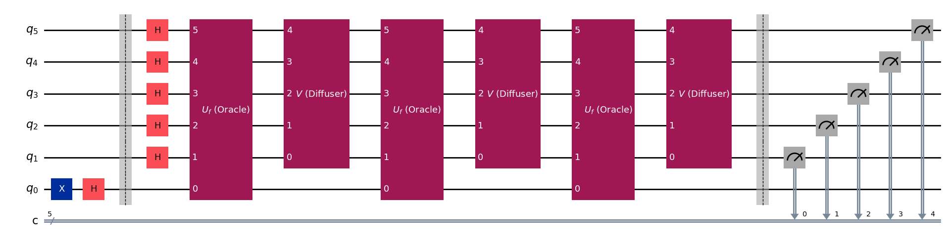
n = 5                                             # Number of qubits
N = 2**n                                          # Number of elements
M = 2                                             # Number of marked elements
κ = round(np.pi/(4*np.arcsin(np.sqrt(M/N)))-1/2)  # Number of iterations

qc, m_lst = grover_M_marked(n, M, κ)
qc.draw(fold=-1)

simulator = AerSimulator()

qc_t = transpile(qc, simulator)
job = simulator.run(qc_t, shots=2**13)
counts = job.result().get_counts()

print(f'Secret marked elements: {m_lst}')
plot_distribution(counts, figsize=(10,5), title='Frequency of measuring each element')

Secret marked elements: ['00101', '01101']