Simon’s Algorithm#
Simon’s algorithm, introduced by Daniel R. Simon in 1994, was the first quantum algorithm shown to solve a problem exponentially faster than the best known classical methods [Simon94].
Although the problem tackled by this algorithm (known as Simon’s problem) has no direct practical relevance, its discovery laid the groundwork for Shor’s algorithm, one of the very few quantum algorithms with a proven advantage for a real-world application.
Simon’s problem is similar to the Bernstein-Vazinari problem in that we are tasked with finding a secret string \(s\). However, the function that encodes \(s\) is different. In Simon’s problem, we are given a function that takes an \(n\)-bit input \(x\) and produces an \(n\)-bit output \(f(x)\) (i.e., \(f: \{0, 1\}^n \longmapsto \{0, 1\}^n\)) where we are promised that \(f(x) = f(s \oplus x)\)\(^*\). Here, \(s\) is an \(n\)-bit string different from \(0\), and \(\oplus\) denotes the bitwise XOR (addition modulo-2) operation:
This condition guarantees that there will be two values of \(x\) for which \(f(x)\) takes the same value. In other words, the function \(f(x)\) is two-to-one. For example, given the string \(s = 110\) a possible valid function \(f: \{0, 1\}^3 \longmapsto \{0, 1\}^3\), has the following associated mapping:
Notice how, for example, for \(x = 001\) and \(x = (110 \oplus 001) = 111,\) we obtain the same \(f(x) = 100.\)
It is worth noting that, for the purpose of Simon’s problem, the value that \(f(x)\) takes for each individual \(x\) is completely arbitrary as long as the condition \(f(x) = f(s \oplus x)\) is met.
Let’s now use python to generate an arbitrary function \(f(x)\) for every possible value of \(x\) given a string \(s\):
import numpy as np
def fx_simon(s_int, n):
    fx_lst = [0]*2**n
    x_used = []
    fx_avail = list(range(2**n))

    for x_int in range(2**n):
        if x_int in x_used: continue

        x_pair = s_int ^ x_int
        x_used.extend((x_int, x_pair))

        # pick random f(x) value and remove from available list
        fx_int = np.random.choice(fx_avail)
        fx_avail.remove(fx_int)

        # assign f(x) value to x and s⊕x
        fx_lst[x_int] = fx_int
        fx_lst[x_pair] = fx_int

    return fx_lst
s = '1101'          # String (pick value different from all-zeros string).
n = len(s)
s_int = int(s, 2)

fx_lst = fx_simon(s_int, n)

print(f'Outcomes for s = {s}\n')
print('x',' '*(n), 'f(x)')

for x_int, fx_int in enumerate(fx_lst):
    x = np.binary_repr(x_int,n)
    fx = np.binary_repr(fx_int,n)

    print(x, ' ', fx)
Outcomes for s = 1101

x      f(x)
0000   0010
0001   1100
0010   1111
0011   1001
0100   0101
0101   0100
0110   0000
0111   1110
1000   0100
1001   0101
1010   1110
1011   0000
1100   1100
1101   0010
1110   1001
1111   1111
Rerunning the cell above will result different values of \(f(x)\) (picked at random) for each corresponding \(x\). However, the condition \(f(x) = f(s \oplus x)\) is always fulfilled.
1. Classical Approach#
To solve Simon’s problem classically, we have to evaluate the function \(f(x)\) for different input values until we get two values of \(x\) that share the same output. If the inputs for which we get the same outcome are the pair \(\{a, b\},\) we know that \(f(a) = f(b).\) Now, since \(f(x) = f(s \oplus x)\) for all values of \(x,\) this implies that \(b = s \oplus a\). We can then find \(s\) by taking the XOR with \(a\) on both sides of this expression:
This equality holds because taking the bitwise XOR of any number with itself is always zero (i.e., \(a \oplus a = 0\)).
So, if we get very lucky, it can take us only \(2\) tries to find repeated outcomes that allows us to extract \(s\) (best case scenario). However, since \(f(x)\) is two-to-one, for a string of length \(n\) there are \(2^n/2 = 2^{n-1}\) possible value of \(f(x)\), so it can take up to \(2^{n-1} + 1\) tries to find two inputs with a matching output (worst case scenario). Later in this section we will explore how the probability of success changes for a given number of tries.
Similar to what we did for the Deutsch-Jozsa and Bernstein-Vazirani problems, we can encode the function \(f(x)\) for Simon’s problem into a unitary \(U_f\) that we can either run as a classical reversible circuit, or use as part of a quantum algorithm:
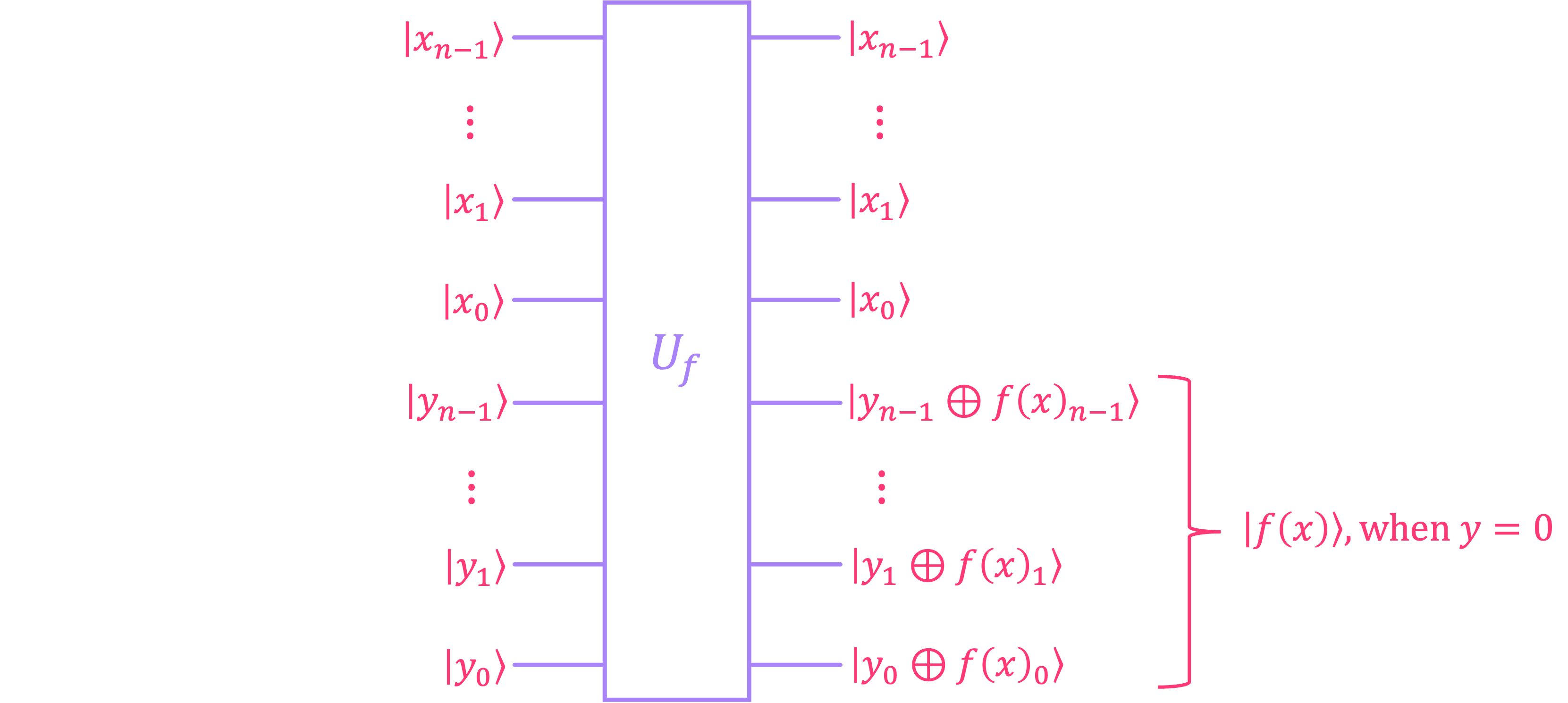
Here, the top \(n\) qubits (labeled \(|x\rangle\)) correspond to the function input, and the bottom \(n\) qubits produce the output \(|f(x)\rangle\) when \(|y\rangle = |0\rangle^{\otimes n}.\)
Let’s now create a python function that naïvely encodes the \(f(x) = f(s \oplus x)\) condition into \(U_f\) (details on this and a more efficient implementation are discussed in section 3).
from qiskit import QuantumCircuit, transpile
from qiskit_aer import AerSimulator
def black_box(n):
    # Black box of Simon's problem using naïve implementation.
    # It encodes it each product element from a sum of products asan MCX gate.
    s_int = np.random.randint(1, 2**n)
    s = np.binary_repr(s_int, n)

    fx_controls = [[] for _ in range(n)]
    fx_lst = fx_simon(s_int, n)

    # Iterate over fx_list where each index is x, value is integer value of fx
    # and find the control values for each fx_i that evaluates to 1.
    for x_int, fx in enumerate(fx_lst):
        for bit, fx_bit in enumerate(reversed(np.binary_repr(fx, n))):
            if fx_bit == '1':
                fx_controls[bit].append(x_int)

    qc_bb = QuantumCircuit(2*n, name='Black Box')
    for i, controls in enumerate(fx_controls):
        for int_ctrl_state in controls:
            ctrl_state = np.binary_repr(int_ctrl_state,n)
            qc_bb.mcx(list(range(n,2*n)),i,ctrl_state=ctrl_state)
        qc_bb.barrier()

    return qc_bb, s
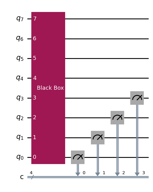
# Draw example circuit to solve B-V's problem classically (n = 4, x = 0000)
n = 4
bb, _ = black_box(n)

qc = QuantumCircuit(2*n,n)
qc.append(bb,range(2*n))
qc.measure(range(n),range(n))
qc.draw()
We can now try each possible classical input \(x\) and check that, for the encoded string \(s\), our unitary \(U_f\) does correctly return a two-to-one function for which the condition \(f(x) = f(s \oplus x)\) holds:
# Go over every input and output

n = 3                        # String length
bb, s = black_box(n)         # Generate black box and secret string
fx_meas = {}                 # Dict where keys are measured fx and values are corresponding x

simulator = AerSimulator()

print(f'Outcomes for s = {s}\n')
print('x',' '*(n), 'f(x)')
for x_int in range(2**n):

    x = np.binary_repr(x_int, n)
    input_ones = [i+n for i, v in enumerate(reversed(x)) if v == '1']

    qc = QuantumCircuit(2*n,n)
    if input_ones: qc.x(input_ones)
    qc.append(bb,range(2*n))
    qc.measure(range(n),range(n))

    qc_t = transpile(qc, simulator)
    job = simulator.run(qc_t, shots=1, memory=True)  # Run one simulation to get f(x) outcome
    fx = job.result().get_memory()[0]

    print(x, ' ', fx)
Outcomes for s = 100

x     f(x)
000   100
001   110
010   001
011   010
100   100
101   110
110   001
111   010
Let us now run a classical procedure to solve Simon’s problem by picking different input values of \(x\) at random until we find two matching values of \(f(x).\) Once found, we can then extract the encoded secret string \(s\) by taking the XOR between the two inputs that produced the matching outputs:
n = 7                        # String length
bb, s = black_box(n)         # Generate black box and secret string

fx_meas = {}                  # Dictionary to store string extracted from f(x) and the corresponding value of x
match = False                 # Has a match been found?
x_avail = list(range(2**n))   # List with all possible x values to try
tries = 0                     # Number of tries to find s

while not match:

    # pick x at random
    x_int = np.random.choice(x_avail)
    x_avail.remove(x_int)
    x = np.binary_repr(x_int, n)

    # evaluate Uf for selected x
    input_ones = [i+n for i, v in enumerate(reversed(x)) if v == '1']

    qc = QuantumCircuit(2*n,n)
    if input_ones: qc.x(input_ones)

    qc.append(bb,range(2*n))
    qc.measure(range(n),range(n))

    qc_t = transpile(qc, simulator)
    job = simulator.run(qc_t, shots=1, memory=True)
    fx = job.result().get_memory()[0]

    tries += 1

    if fx in fx_meas:
        s_out = np.binary_repr(x_int ^ int(fx_meas[fx], 2), n)
        match = True
    else:
        fx_meas[fx] = x

print(f'secret string: {s}')
print(f'extracted string: {s_out}')
print(f'number of tries: {tries} (out of {int(2**n/2)} possible outputs)')
secret string: 1011111
extracted string: 1011111
number of tries: 6 (out of 64 possible outputs)
Rerunning the cell above will always extract the secret string correctly, but the number of tries it’ll take will vary.
Calculating the probability of finding a secret string of length \(n\) after a certain number of tries \(r\), is akin to solving the birthday paradox problem, but where the sample space changes as a function of the number of extracted values \(k\):
The details of how this expression is obtained are out of the scope of our discussion. What’s critical here, is that this equation shows that for a string of length \(n\), it takes roughly \( r \sim \sqrt{2^{n}} = 2^{n/2}\) tries to find \(s\) with more than \(50 \%\) probability. This means that with a classical approach, the number of tries needed to successfully find \(s\) with high probability grows exponentially with the length of the string \(n.\)
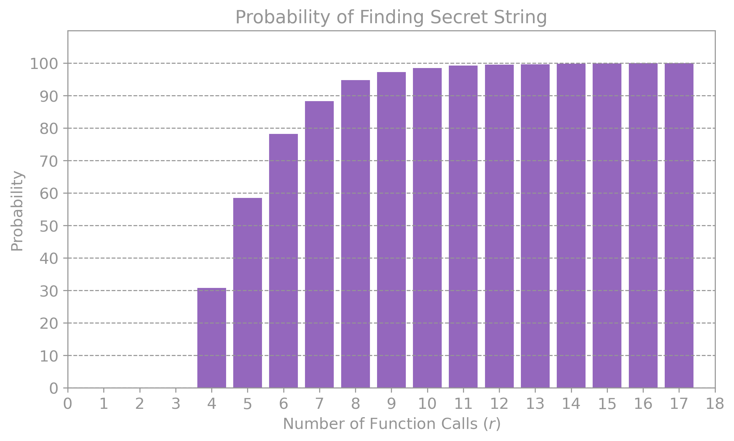
The plot below shows the simulation result for the probability of finding a secret string of length \(n = 5\) after a certain number of tries \(r:\)
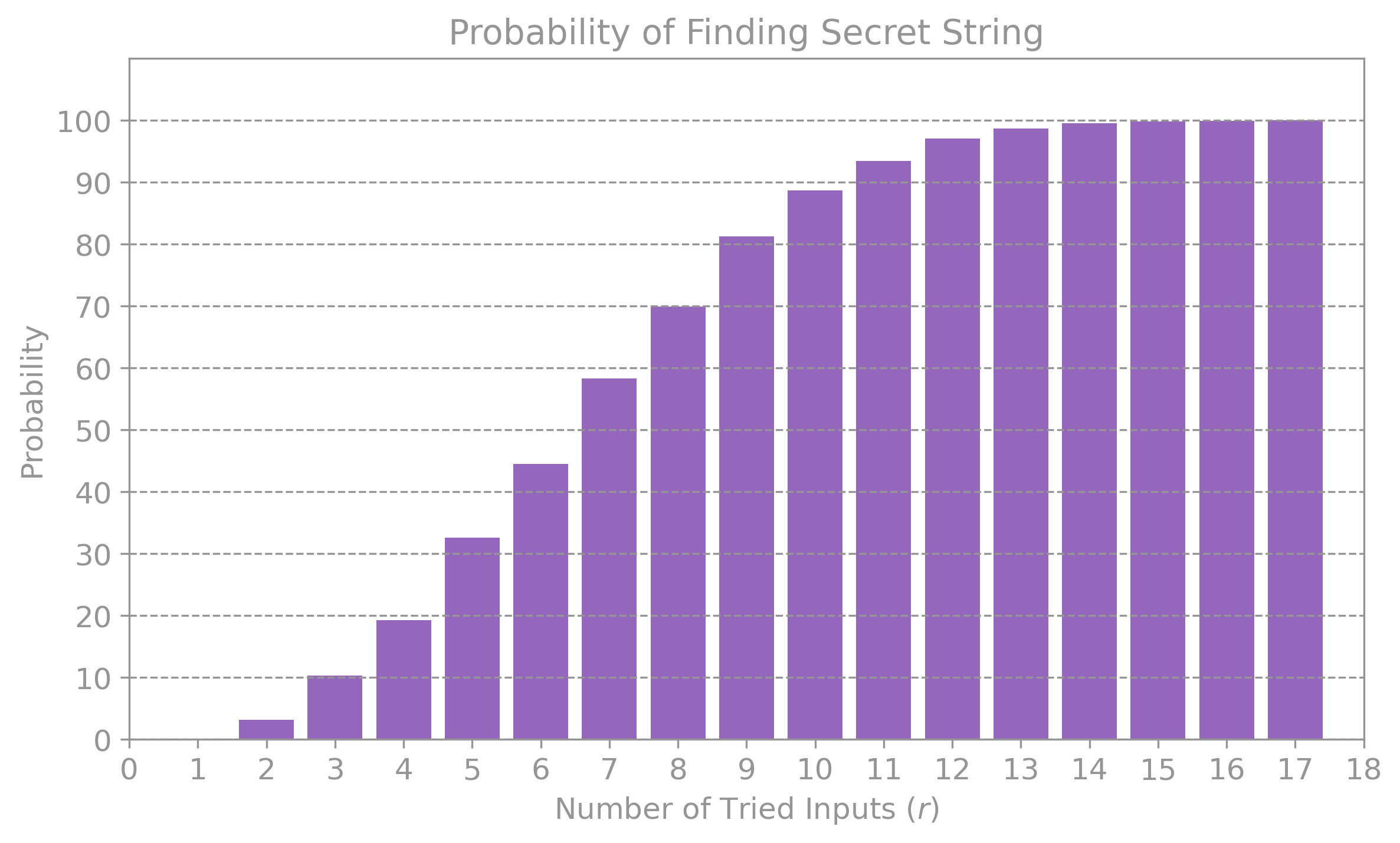
It can be seen that only after \(r = 6\) tries, the probability of success is over \(50 \%,\) which is close to the expectation of requiring a value larger than \(2^{5/2} \approx 5.66.\)
2. Quantum Approach#
In contrast to the Deutsch-Jozsa and Bernstein-Vazirani algorithms (which yield a solution in a single try), Simon’s algorithm requires multiple accesses to the unitary \(U_f\) in order to determine the secret string \(s\) with high probability. However, unlike the classical approach we described above (which needs a number of function evaluations that grows exponentially with \(n\)), Simon’s algorithm only requires an average number of calls to \(U_f\) that grows linearly with \(n.\) Furthermore, will see that, in contrast to previous quantum algorithms, Simon’s algorithm relies on classical post-processing steps, where the measurement outcomes of multiple quantum circuit runs are used to compute \(s.\)
2.1 Quantum Circuit#
The quantum circuit utilized in Simon’s algorithm is similar to that of the Deutsch-Jozsa and Bernstein-Vazinari algorithms in that we place the top register \(x\) in superposition, evaluate \(U_f,\) and then perform interference.
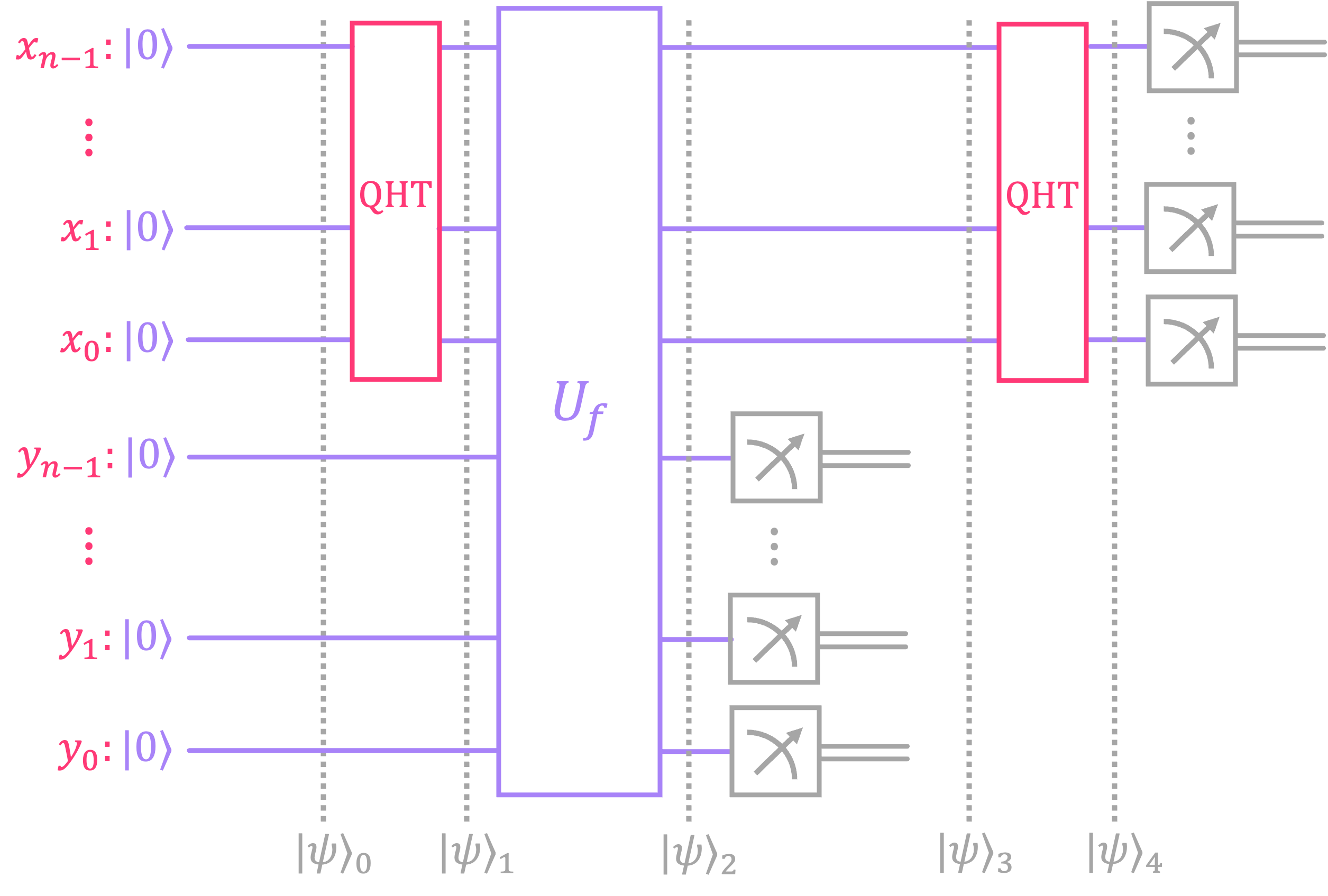
However, the circuit is different in that we do not prepare the bottom register \(y\) in an eigenstate of \(U_f\) to perform phase kickback. Instead, we initialize them in the all-zeros state \(|0\rangle^{\otimes n}\) and measure them right after the function evaluation takes place.
To understand the reasoning for this approach, lets analyze the circuit step by step for an arbitrary number of bits \(n\). In section 2.3 we will go over a concrete example using 3 qubits to clarify the process.
Initialize both qubit registers in the all-zeros state:
Place top register \(x\) in a uniform superposition:
Evolve the state over \(U_f\):
Here, \(|\psi\rangle_2\) is a superposition state over all possible \(|x\rangle\) values and their corresponding \(|f(x)\rangle\). Now, since our function meets the condition \(f(x) = f(s \oplus x),\) we know that every state \(|x\rangle\) will have a corresponding \(|s \oplus x\rangle\) that shares the same \(|f(x)\rangle.\) Therefore, we can rewrite the expression above as:
where \(S\) is a subset of all possible values of \(x\) that only contains elements that evaluate to unique values of \(f(x)\) (and therefore depends on the string \(s\)).
Next, we measure the bottom register \(y,\) which will cause the superposition state \(|\psi\rangle_2\) to be projected onto a state with a single value of \(f(x).\) Let’s call this state \(|f(a)\rangle,\) where \(a\) is some arbitrary value of \(x.\) This leaves the top register \(x\) in a superposition of the two states that evaluate to the same \(f(a)\):
For the remaining of the analysis, we can drop the state of the bottom register since it has already been measured, leaving us with \( |\psi\rangle_3 = \frac{1}{\sqrt{2}} \left(|a\rangle + |s\oplus a\rangle \right).\)
We perform interference by applying the \(\text{QHT}\) to the top register:
If we now focus on the probability amplitude expression inside the square brackets, we see that we have two possibilities:
if \((s \cdot z) = 1,\) then \(\left[1 + (-1)^{s \cdot z} \right] = 0, \)
if \((s \cdot z) = 0,\) then \(\left[1 + (-1)^{s \cdot z} \right] = 2 .\)
What this means is that, all the \(|z\rangle\) terms in the summation for which the dot product between \(s\) and \(z\) is \(1\), vanish. This leaves us with a state where only the terms for which \(s \cdot z = 0\) survive:
Here it is worth noting that, regardless of the value of the string \(s\), the expression \(s \cdot z = 0\) always holds for \(z = 0\). Therefore, one of the terms that is always present in the superposition is the all-zeros string \(|z\rangle = |0\rangle^{\otimes n}.\) As a matter of convenience, we can pull this term out from the summation to make this explicit:
The final step in the circuit is to measure state \(|\psi\rangle_4\), which produces one of two types of outcomes:
With probability \(\left|\frac{1}{\sqrt{N/2}}\right|^2 = \frac{2}{N},\) we measure the all-zeros string \(|0\rangle^{\otimes n}.\)
With probability \(1 - \frac{2}{N},\) we measure some other state \(|z\rangle\) for which the equation \(s \cdot z = 0\) holds.
The first case is considered a “failed” attempt since it gives us no information whatsoever about the string \(s.\) This means that, if we execute the circuit and measure \(z = 0 \dots 00,\) we need to re-run the circuit.
The second case, on the other hand, provides us with a classical binary string \(z = z_{n-1} ... z_1 z_0\) that meets the condition:
This basically corresponds to a linear equation (modulo 2), where each \(z_i\) is a coefficient equal to \(0\) or \(1,\) and each \(s_i\) is an unknown variable. We can then execute Simon’s quantum circuit several times to extract different values of \(z\) that allow us to form a system of \(n-1\) linearly-independent equations:
Here, the superscripts \(j\) \(\big(\)in \(z^{(j)} \big)\) are used to represent the different \(z\) strings measured after executing the quantum circuit. Solving this system of equations gives us as a solution the \(n\) bits of \(s.\)
As mentioned before, every time we measure the all-zeros string or get a repeated value of \(z\), we must re-execute the circuit. However, since we only need \(n - 1\) equations to find \(s\), the number of calls will be much smaller (linear in \(n\)) compared to the number of calls we needed classically (exponential in \(n\)).
Therefore, in addition to executing the quantum circuit, we also need a procedure that:
verifies that every measured \(z\) is not the all-zeros string or a repeated value of \(z\),
checks that every new \(z\) is linearly-independent from previous measured values (explained in the next section),
stores every valid \(z\) until we have \(n-1\) results,
and solves the resulting linear system of equations.
Let’s cover these steps in more detail in the next section.
2.2 Classical Post-Processing#
From the explanation above, it is clear that Simon’s algorithm requires a combination of quantum and classical steps. As a matter of fact, the flow chart below shows that the quantum circuit is only a portion of a larger hybrid process:
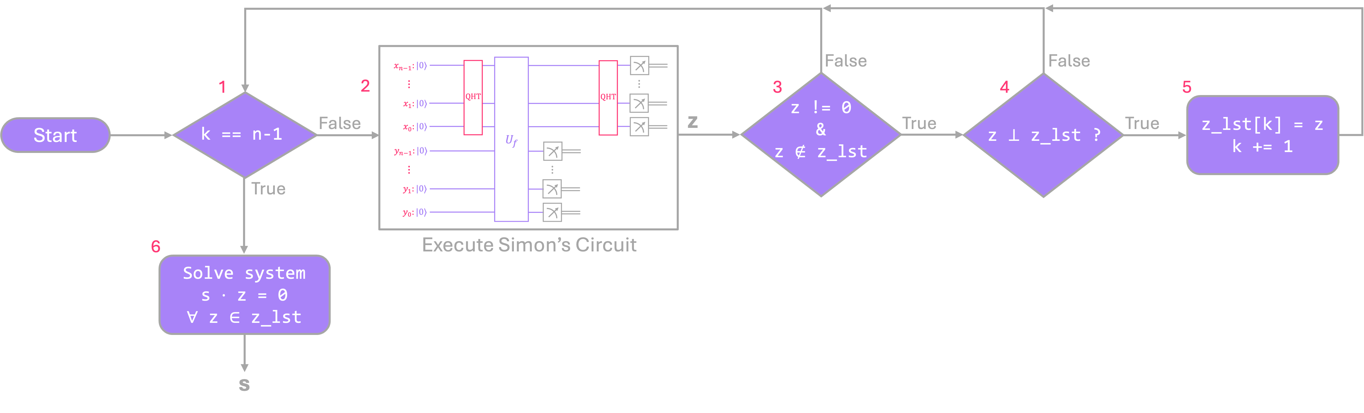
Let’s go over each of the steps:
The algorithm starts by checking if the number of stored
zoutputs (tracked by the valuek) is already equal to the minimum number of linearly-independent equations (n - 1) required to find thenbits of the strings.If the condition above is not met, Simon’s circuit is executed to extract a new output
z.The next step checks if the circuit outcome
zis not the all-zeros string and is not already in the list of stored valuesz_lst. If these conditions are met, the algorithm proceeds. If it fails, the circuit must be rerun.Next, it must be verified if
zis linearly-independent from all previous values stored inz_lst(more on this below). If not, the circuit must be re-executed.If step 4 passes,
zis stored inz_lstandkis incremented. All steps above must be repeated untilk = n - 1.Once all necessary values of
zare available, the algorithm proceeds to solve the linear system of equations and finds.
Steps 1, 2, and 3 were described in detail in the previous section, so we can now focus on the classical post-processing steps involved in finding the \(n - 1\) linearly-independent equations, and solving the system to find \(s\).
Now, the reason why we check for linear independence is because, an equation generated by a value of \(z\) that can be expressed as a linear combination of previous results, doesn’t provide any new information about how to solve for \(s\). However, let’s start by first analyzing the case where, instead of checking right away if every new outcome is linearly independent from previous ones, we collect \(m\) unique values of \(z\), where \(m\) much larger than the required \(n-1\) linearly-independent equations. In other words, we skip step 4 altogether and collect many samples of \(z\) with the hope that \(n - 1\) of these will generate linearly-independent equations. Now, even if some of our outcomes are not linearly independent, we know that each of them still generate an equation of the form \(z^{(j)} \cdot s = 0: \)
We can rewrite this expression as the dot product (modulo 2) of two binary vectors \(\vec{z}^{(j)}\) and \(\vec{s},\) where their entries are the bits of \(z\) and \(s\), respectively: \(\vec{z}^{(j)} \cdot \vec{s} = 0 .\) Written in vector form:
We can then organize the \(m\) different equations by stacking each \(\vec{z}^{(j)}\) as rows in a matrix:
This expression is of the form \(Z \vec{s} = \vec{0},\) which is convenient because it allows us to use linear algebra techniques to find the unknown vector \(\vec{s}.\) More explicitly, \(\vec{s}\) can be found by computing the kernel of the matrix \(Z.\) Here, the kernel is nothing other than the group of vectors that, when multiplied by \(Z,\) result in the all-zeros vector. In other words, the elements in the kernel of \(Z\) correspond to the vectors \(\vec{s}\) that solve the expression above.
The first step to compute the kernel of a matrix, is to express it in what is known as its reduced row echelon form (RREF) through Gauss-Jordan elimination. Here we won’t focus on the details of how this is done; all we need to know is that, if our \(m\) collected samples of \(z\) contain \(n - 1\) values that are linearly-independent, the RREF of \(Z\) will be a matrix where the first \(n-1\) rows correspond to a set of new basis vectors \(\vec{\zeta}^{(j)},\) and the remaining \( m - (n - 1) \) rows are all \(0:\)
In the end, the basis vectors \(\vec{\zeta}^{(j)}\) will form the \(n - 1\) linearly independent expressions we need to solve for \(\vec{s}\).
Now, selecting an optimal value for \(m\) can be tricky because, if we pick it to be too small, there is a chance that we will not obtain the \(n - 1\) linearly-independent values of \(z\) we need to solve the system of equations. On the other hand, if we pick it too large, we can end up with several linearly-dependent samples, which do not provide us any additional basis vectors \(\vec{\zeta}.\) So what we can do, is compute the basis vectors on the fly. Every time we sample a new \(z\) from our circuit, we perform Gaussian elimination. If the process results in a new basis vector, we store it; if not, we execute the circuit again to obtain a new \(z\) and repeat the process until we have the \(n - 1\) basis vectors we need. These are basically steps 4 and 5, so all we have left is to perform step 6, which entails solving for \(\vec{s}\) in the vector equation \(Z\vec{s} = \vec{0}\) via back-substitution, but where we replace the matrix \(Z\) with its corresponding RREF:
Let’s now take a look at a concrete numerical example of the full algorithm to get a better understanding of how each step works.
2.3 Numerical Example#
Let’s start by assuming that we are given access to a unitary \(U_f\) which encodes a function \(f(x).\) We are promised that function satisfies the condition for Simon’s problem \(f(x) = f(s \oplus x)\) for a secret string \(s = 1010,\) and has the following input/output relation:
2.3.1 Quantum Circuit Analysis#
Since \(x\) and \(f(x)\) encode \(4\) bits each, the unitary \(U_f\) that encodes the function (and therefore, our quantum circuit) must have a total of \(8\) qubits. Let’s go over each of the steps we described in section 1.2.1:
Initialize the circuit qubits in the all-zeros state:
Apply the \(\text{QHT}\) to place top register in a uniform superposition:
writing out each term explicitly:
Evolve the state through \(U_f,\) which basically pairs up each \(|x\rangle\) with its corresponding \(|f(x)\rangle\) (given in the table above).
Measure the bottom register, which projects the state onto a single value \(|f(a)\rangle\) and places the top register in a superposition of \(|x\rangle\) and \(|s \oplus x\rangle .\) Let’s assume that, after the first execution, the measured value was \(f(a) = 1011,\) resulting in the state:
Apply the \(\text{QHT}\) on the top register:
At this point it is worth pausing to highlight that, when we rerun the circuit, step 3 will likely result in a measurement that returns a different value of \(f(x)\). However, the superposition we obtain in step 4 will always be composed by the same basis states, just with different relative phases! This is because Simon’s circuit is designed to always result in a superposition of states \(|z\rangle\) that meet the condition \(s \cdot z = 0,\) independent of the measured value \(f(x).\) For example, let’s assume that after a executing the circuit again, in step 3 we measure \(f(b) = 1110,\) resulting in the following state:
Applying the \(\text{QHT}\) on the top register gives us:
which has the same components we obtained in the first run.
So, independent of what value of \(f(x)\) we measure, the state we get in step 4 is always a superposition of the same components: \(\{|0000\rangle,\) \(|0001\rangle,\) \(|0100\rangle,\) \(|0101\rangle,\) \(|1010\rangle,\) \(|1011\rangle,\) \(|1110\rangle,\) \(|1111\rangle \}.\)
The last step in the quantum circuit is to measure the top register, which will result in either:
The string \(z = 0000\) with probability \(|\frac{1}{\sqrt{8}}|^2 = \frac{1}{8},\) providing no information about the secret string \(s.\)
A \(z\) string from the list \(\{0001,\) \(0100,\) \(0101,\) \(1010,\) \(1011,\) \(1110,\) \(1111\}\) with probability \(\frac{7}{8},\) which we can use in the classical post-processing steps to extract \(s\).
2.3.2 Classical Processing Analysis#
From the analysis above, we know that every time we run the quantum circuit we get one of the following outcomes:
Lets assume that after the first run, we obtain outcome: \(z^{(1)} = 0001.\) This gives us our first linear equation:
We run the circuit again and obtain \(z^{(2)} = 1010,\) with a corresponding equation:
We run the circuit a third time and get \(z^{(3)} = 1011,\) which results in:
Since this equation is a linear combination of the previous two, it gives us no new information to solve for \(s\) (since we already knew that \(s_3 \oplus s_1 = 0\) and \(s_0 = 0\)). We then need to get a new sample from the quantum circuit.
A fourth run returns outcome \(z^{(4)} = 1110,\) with equation:
Given that we know \(s_3 \oplus s_1 = 0,\) this guarantees that \(s_2 = 0.\) This also reveals that \(s_3\) and \(s_1\) must both equal \(1\) because if they were both \(0,\) the string \(s\) would be the all-zeros string, which we know is not an allowed solution.
This reveals that our secret string is \(s = 1010,\) as expected.
So far, we explained the post-processing steps in an intuitive way tracking each of the obtained equations. But we can also follow the procedure covered in section 1.2.2, where we find a series of \(n - 1\) basis vectors \(\vec{\zeta}\) and solve a matrix equation.
In the first step above we obtained \(z^{(1)} = 0001.\) Since we don’t have any other basis vectors yet, we store it:
NOTE: In the vector notation we’ve followed so far, we place the least significant bit of \(z\) as the first vector element. That’s why the order might seem reversed.
The second step gave the value \(z^{(2)} = 1010.\) We then stack this and the previous stored vector on a matrix and perform Gaussian elimination. Now, since \(z^{(2)}\) is linearly-independent from \(\vec{\zeta}^{(1)},\) we find that new basis vector that is identical to \(\vec{z}^{(2)}\), so we store it:
In the third run, we got \(z^{(3)} = 1011,\) which is a linear combination of \(\zeta^{(1)}\) and \(\zeta^{(2)}.\) So, if we were to run Gaussian elimination between \(\vec{\zeta}^{(3)}\) and the basis vectors \(\vec{\zeta}^{(1)}, \vec{\zeta}^{(2)},\) we will get an all-zeros vector, which we discard.
Lastly, in the fourth run, we obtained \(z^{(4)} = 1110.\) Running Gaussian elimination between \(\vec{z}^{(4)}\) and \(\vec{\zeta}^{(1)}\), \(\vec{\zeta}^{(2)}\), results in a new basis vector:
We now have the \(n - 1 = 3\) basis vectors we need to form our RREF matrix and solve for \(s:\)
As expected, we get the string \(s = 1010.\)
2.4 Python Implementation#
First, let’s create a function that generates Simon’s quantum circuit:
def simons_cir(n):
    bb, s = black_box(n)                     # generate random black-box of n input qubits

    qc_s = QuantumCircuit(2*n,2*n)
    qc_s.h(range(n,2*n))                     # Hadamard gates top n qubits
    qc_s.append(bb,range(2*n))               # append black box to circuit
    qc_s.measure(range(n),range(n))          # measure bottom n qubits
    qc_s.barrier()
    qc_s.h(range(n,2*n))                     # Hadamard gates on top n qubits
    qc_s.measure(range(n,2*n),range(n,2*n))  # measure top n qubits

    return qc_s, s
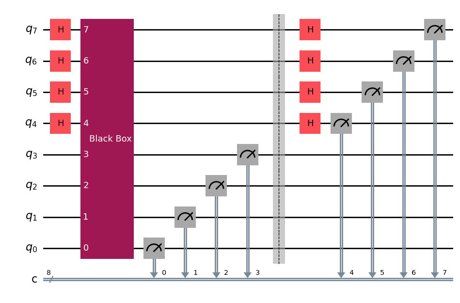
# Draw example of Simon's circuit for 4 qubits
qc = simons_cir(4)[0]
qc.draw()
In addition to the quantum circuit, we need two classical helper functions. The first one (generate_basis), checks that if output of the circuit is a value that is linearly independent from previous results, and generates an updated list of basis vectors that includes the new reduced vector.
The second function (kernel_from_basis) is used to compute the secret string \(s\) by finding the kernel of the matrix that contains as its rows the \(n - 1\) basis vectors obtained from the previous steps.
def generate_basis(basis: list[int], z: int):
    # Returns updated list of binary basis vectors by reducing a new entry `z` through
    # Gaussian elimination (mod 2). For convenience, we treat each "vector" as an integer,
    # where the bits of its binary representation correspond to the elements of the vector.

    basis = basis.copy()

    # Reduce z using existing pivots
    for b in basis:
        p = (b & -b).bit_length() - 1   # finds index of the lsb that's equal to 1 (pivot)
        if (z >> p) & 1:                # checks if the p^th bit of z is 1
            z ^= b                      # reduce z by XOR with basis vector b

    if z == 0: return basis             # If reduced z is zero, it was dependent
    p = (z & -z).bit_length() - 1       # finds index of the lsb that's equal to 1 (pivot)


    # Eliminate pivot from existing basis vectors (now z contains it)
    for i, b in enumerate(basis):
        if (b >> p) & 1:
            basis[i] ^= z

    basis.append(z)
    return basis
def kernel_from_basis(basis: list[int], n:int):
    # Returns the secret string s: int, which is the kernel of the RREF matrix
    # containing the basis vectors in `basis`. n is the number of bits in the secret string.
    # For convenience, we treat each "vector" as an integer, where the bits of its
    # binary representation correspond to the elements of the vector.

    # Find pivot positions
    pivots = []
    for b in basis:
        if b == 0:
            continue
        p = (b & -b).bit_length() - 1  # finds index of the lsb that's equal to 1 (pivot)
        pivots.append(p)

    pivot_set = set(pivots)

    # Find free positions
    free_positions = [j for j in range(n) if j not in pivot_set]

    # Build kernel vectors
    kernel_basis = []
    for free in free_positions:
        s = 1 << free  # set free variable to 1

        # solve pivot variables
        for b, p in zip(basis, pivots):
            if (b >> free) & 1:
                s ^= (1 << p)

        kernel_basis.append(s)

    return kernel_basis
We can now put everything together by combining the quantum circuit with the classical-post processing steps:
n = 7            # Length of secret string s
k = 0            # Number of linearly-independent values found
tries = 0        # Number of tries to find s
basis_vects = [] # List of vectors representing system of linear equations

simulator = AerSimulator()

qc_s_cir, s = simons_cir(n)   # Generate Simon's circuit for a random string s

while k < n - 1:

    # transpile and run quantum circuit
    qc_t = transpile(qc_s_cir, simulator)
    job = simulator.run(qc_t, shots=1, memory=True)
    z_and_fx = job.result().get_memory()[0]   # returns results for both top and bottom registers
    z = int(z_and_fx[0:n], 2)                 # extract z only (as integer)

    if z != 0:
        basis_vects = generate_basis(basis_vects, z)
        k = len(basis_vects)

    tries += 1

s_out = np.binary_repr(kernel_from_basis(basis_vects, n)[0],n)

print(f'secret string: {s}')
print(f'extracted string: {s_out}')
print(f'number of tries: {tries} (out of {int(2**n/2)} possible outputs)')
secret string: 0111010
extracted string: 0111010
number of tries: 7 (out of 64 possible outputs)
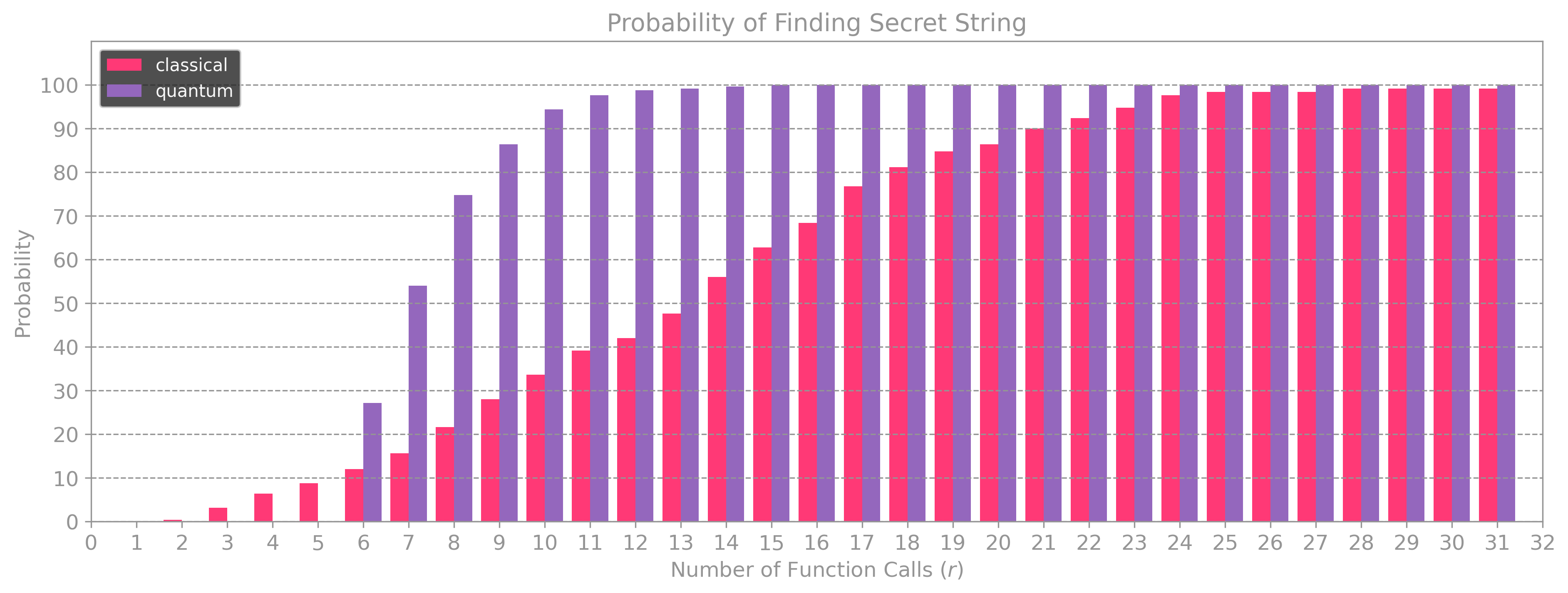
Even for small values of \(n\), we can check that the quantum algorithm performs better than its classical counterpart by running the code above and computing the probability of success for a given number of tries \(r\). The plot below shows the results for a simulation with \(n = 5,\) which compared to the plot in section 1.1 provides a much higher probability of success at lower values of \(r.\)
It is also worth noting that for the quantum algorithm, the probability of success will always be zero for \(r < n - 1\) because we need to collect at least \(n - 1\) samples to solve the linear system of equations. When placing the results for the classical and quantum algorithms this difference becomes obvious. For \(n = 7,\) the probability of success for the quantum algorithm is \(0\) before \(r = 6\), but after that, it passes the \(50 \%\) mark at \(r = 7 .\) In contrast, the classical approach requires \(r = 14\) tries to succeed more than \(50 \%\) of the time.
Footnotes#
\(^*\)The definition of Simon’s problem is actually broader than what is described above. More generally, Simon’s problem considers an \(n\) to \(m\) function \(f: \{0, 1\}^n \longmapsto \{0, 1\}^n, \, m \geq n,\) which meets the condition \(f(x) = f(s \oplus x).\) The function is either one-to-one (when \(s\) is the all-zeros string) or two-to-one (when \(s\) is any other string). Simon’s decision problem consists of finding which of these two types of function \(f(x)\) is. Simon’s no-decision problem consists in finding what the bit-string \(s\) is, which is what is described in this chapter for the case in which \(m = n.\) (go back)
3. Comments on Black Box Implementation#
In this section, we will discuss the details of how to implement the unitary \(U_f\) that encodes the function for Simon’s problem \(f(x) = f(s \oplus x)\).
Let’s consider the most general case in which, instead of getting an explicit Boolean function, we are given the input/output (Truth Table) for the bits of \(f(x).\) For example, we are given the following relation:
This truth table corresponds to a function that meets the constraint \(f(x) = f(s \oplus x)\) when s = \(100.\)
To construct the circuit for the unitary \(U_f\), we will need two 3-qubit registers; one for the input bits \(x_0, x_1, x_2\) and one to evaluate the outputs \(f(x)_0, f(x)_1, f(x)_2.\)
We can then use a simple approach and first find the Boolean expressions for each output \(f(x)_i\) that evaluates to \(1\) as a sum of products (i.e., find the Disjunctive normal form (DNF) by semantic means):
Next, all we need to do is add to our circuit one \(MCX\) gate per product term in each of the expressions. For example, \(f(x)_0,\) has two product terms, so we need two \(MCX\) gates with their target on the \(0^{th}\) qubit of the register where \(f(x)\) is evaluated, and their control conditioned on the values of \(x\) that make the expression evaluate to \(1\). Here’s how the circuit will look like for \(f(x)_0\):
This circuit guarantees that when \(x\) is either ‘011’ or ‘111’, qubit \(y_0\) will evaluate to \(f(x)_0 = 1.\) All that’s left is to repeat this process for \(f(x)_1, f(x)_2:\)
Let’s confirm that this circuit does return the expected values of \(f(x)\) for each input \(x:\)
The function
black_boxthat we defined in section 1, performs the same steps we described above but for a random Simon’s function (generated byfx_simon) with an arbitrary number of qubits.The issue with this approach is that it generates very inefficient circuits. Since we didn’t simplify any of the Boolean expressions extracted from the truth table, we end up with either redundant \(MCX\) gates, or with gates that have unnecessary control signals. For instance, in the example above, the expression for \(f(x)_0\) can be simplified as:
This means that, instead of needing two 3-control \(MCX\) gates, we can perform the same operation with one 2-control unitary.
Ideally, a good circuit transpiler should be able to simplify these circuits for us; unfortunately, the current qiskit transpiler is not capable of doing this automatically. So we can either create our own function to perform these simplifications, or use a python library like
sympyto do the job. Let’s go over an example using the same \(f(x)\) we defined above:Now we have 3 simplified expressions for \(f(x),\) but they are in symbolic form! We will need to turn them back into strings of zeros and ones to define the control signals of our \(MCX\) gates. Furthermore, there could be situations in which an expression always evaluates to \(1\) or \(0,\) which means we will need logic to decide when to add an \(MCX,\) an \(X,\) or no gate at all. Fortunately, we can avoid this by using qiskit’s
BitFlipOracleGatewhich takes a function as a input string, and produces the black box we need:If we look inside each of the
BitFlipOracleGategates, we can see the complete simplified black box circuit:Finally, we can modify the original
black_boxfunction from section 1 to generate more efficient black box circuits that run faster for large numbers of qubits: