Bernstein–Vazirani Algorithm

---

The Bernstein-Vazirani algorithm, introduced by Ethan Bernstein and Umesh Vazirani in 1997 [Bernstein97], is a quantum algorithm that, in a single try, solves the Bernstein-Vazirani problem, which entails finding a secret binary string \(s\). In contrast, a classical approach requieres up to \(n\) tries, where \(n\) is the length of the secret string.

The steps of the Bernstein-Vazirani algorithm are identical to those used in the Deutsch-Jozsa algorithm. The difference between the two is in the “black box” \(U_f\), which instead of being either a balanced or constant \(f(x)\), it encodes a function that depends on both the input \(x\) and the string \(s.\)

Concretely, we are given a function of the form \(f(x) = s \cdot x\), where \(x\) and \(s\) are \(n\)-bit binary numbers, and the symbol \(\text{"} \cdot \text{"}\) represents the binary dot product:

\[ s \cdot x = \bigoplus_{i=0}^{n-1} s_{i} x_{i} = s_{0} x_{0} \oplus s_{1} x_{1} \oplus \dots \oplus s_{n-1} x_{n-1} .\]

In other words, we take the bitwise AND (product) between each bit of \(s\) and \(x\), and perform an XOR (addition modulo-2) to get a single output bit \(f(x)\).

Let’s use python to generate each output \(f(x)\) for every possible value of \(x\) given a string \(s\):

import numpy as np

s = '1101'          # String
n = len(s)
s_int = int(s, 2)

print(f'Outcomes for s = {s}\n')
print('x',' '*(n), 'f(x)')

for x_int in range(2**n):    
    x = np.binary_repr(x_int,n)
    fx = sum(int(si,2) & int(xi,2) for si, xi in zip(s, x)) % 2
    
    if x_int == 0 or (x_int & (x_int - 1)):
        print(x, ' ', fx)
    else:
        print(x, ' ', fx, '←')

Outcomes for s = 1101

x      f(x)
0000   0
0001   1 ←
0010   0 ←
0011   1
0100   1 ←
0101   0
0110   1
0111   0
1000   1 ←
1001   0
1010   1
1011   0
1100   0
1101   1
1110   0
1111   1

1. Classical Approach

An interesting observation from the list above is that, whenever we have an input \(x\) where only one of its bits \(x_i\) is equal to \(1\) (elements marked with \(\leftarrow\)), we get an output \(f(x)\) equal to \(0\) if the string \(s\) has the corresponding bit \(s_i\) equal to 0, and an output \(f(x)\) equal to \(1\) if \(s_i = 1\).

So, to extract the string \(s\) from the function \(f(x)\), we can pass each of the following \(n\) possible inputs through \(f(x)\):

\[\begin{split} \begin{aligned} x =&\, 0 \dots 01 \\ x =&\, 0 \dots 10 \\ &\vdots \\ x =&\, 1 \dots 00 , \end{aligned} \end{split}\]

and use each the output to identify the corresponding bit \(s_i\) . In other words, the values of \(x\) shown above serve as individual masks that extract each of the bits of \(s\).

Let’s now create a python function that encodes the function function \(f(x) = s \cdot x\) into a unitary black box \(U_f\) (details on this implementation are discussed in section 1.3).

from qiskit import QuantumCircuit, transpile
from qiskit_aer import AerSimulator

# Function that generates Uf, which encodes f(x) = s⋅x for a random sting s of length n
def black_box(n):
    s_int = np.random.randint(2**n)
    s = np.binary_repr(s_int, n)
    controls = [i+1 for i, v in enumerate(reversed(s)) if v == '1']
    
    qc_bb = QuantumCircuit(n+1, name='Black Box')
    if controls:
        qc_bb.cx(controls,[0]*len(controls))
        
    return qc_bb, s

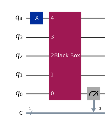
# Draw example circuit to solve B-V's problem classically (n = 4, x = 1000)
n = 4
bb, _ = black_box(n)

qc = QuantumCircuit(n+1,1)
qc.x(n)
qc.append(bb,range(n+1))
qc.measure(0,0)
qc.draw()

If we now iterate over the \(n\) inputs for which \(x\) has only one of it’s bits equal to \(1\), we can find the randomly encoded secret string \(s\) by checking each of the corresponding \(f(x)\) outputs:

n = 3                  # String length
bb, s = black_box(n)   # Generate black box and secret string

s_out = ''             # variable to store string extracted from f(x) classically

simulator = AerSimulator()

for i in range(n):
    
    x_int = 2**i
    x = np.binary_repr(x_int, n)
    input_ones = [i+1 for i, v in enumerate(reversed(x)) if v == '1']
    
    qc = QuantumCircuit(n+1,1)
    qc.x(input_ones)
    qc.append(bb,range(n+1))
    qc.measure(0,0)
    
    qc_t = transpile(qc, simulator)
    job = simulator.run(qc_t, shots=1, memory=True)  # Run one simulation to get f(x) outcome
    outcome = job.result().get_memory()[0]
    
    s_out = outcome + s_out
    
print(f'secret string: {s}')
print(f'extracted string: {s_out}')

secret string: 011
extracted string: 011

We can then conclude that, with a classical approach, it takes exactly \(n\) function evaluations to find the secret string.

2. Quantum Approach

As mentioned before, the quantum algorithm to solve this problem is identical to the Deutsch-Jozsa algorithm, but where our black box \(U_f\) now encodes the function \(f(x) = s \cdot x :\)

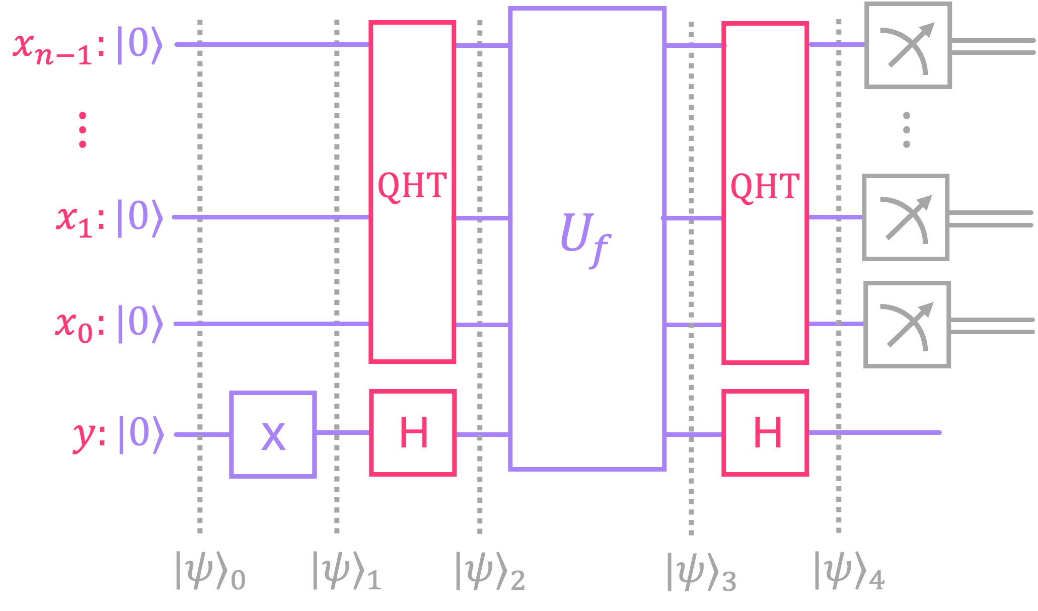
Let’s then analyze the circuit step by step to see the difference:

0. Initialize the all-zeros state: \(|\psi\rangle_0 = |0\rangle^{\otimes n} \otimes |0\rangle\)

1. Apply \(X\) gate to bottom qubit \(y\): \(|\psi\rangle_1 = |0\rangle^{\otimes n} \otimes |1\rangle\)

2. Apply \(H\) gate to qubit \(y\) and \(\text{QHT}\) to register \(x\): \(|\psi\rangle_2 = \text{QHT}_n |0\rangle^{\otimes n} \otimes H |1\rangle\)

This places the to register in an equal superposition over all possible values of \(x\), and the bottom qubit \(y\) in the minus state:

\[ |\psi\rangle_2 = \left( \frac{1}{\sqrt{N}} \sum_{x = 0}^{N - 1} |x\rangle \right) \otimes |-\rangle, \; \text{where} \; N = 2^n . \]

3. Evolve the state through the black box: \(|\psi\rangle_3 = U_f |\psi\rangle_2\), which results in:

\[\begin{split} \begin{aligned} |\psi\rangle_3 &= \left( \frac{1}{\sqrt{N}} \sum_{x = 0}^{N - 1} (-1)^{f(x)} |x\rangle \right) \otimes |-\rangle \\ \\ |\psi\rangle_3 &= \left( \frac{1}{\sqrt{N}} \sum_{x = 0}^{N - 1} (-1)^{s \cdot x} |x\rangle \right) \otimes |-\rangle . \end{aligned} \end{split}\]

Now, the term inside the parenthesis is something we have seen before! This is nothing other than the \(\text{QHT}\) applied to a basis state \(|s\rangle\). We can therefore rewrite \(|\psi\rangle_3\) as:

\[ |\psi\rangle_3 = \left( \text{QHT}_n |s\rangle \right) \otimes |-\rangle . \]

4. Lastly, we apply an \(H\) gate to the bottom qubit \(y\), and the \(\text{QHT}\) to the top register \(x\):

\[\begin{split} \begin{aligned} |\psi\rangle_4 &= \text{QHT}_n \left( \text{QHT}_n |s\rangle \right) \otimes H |-\rangle . \\ \\ |\psi\rangle_4 &= |s\rangle \otimes |1\rangle. \end{aligned} \end{split}\]

This means that, if we measure register \(x\), we will get the string \(s\) with \(100 \%\) probability!

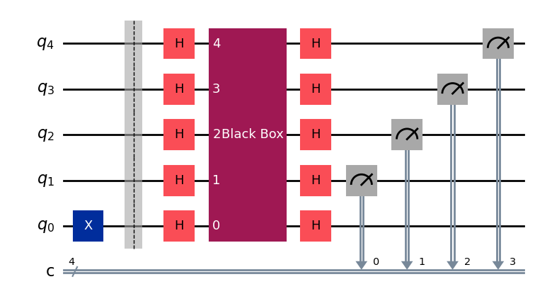
Let’s run this using Qiskit and show that we only need to evaluate the circuit once to extract the secret string \(s.\)

def bernstein_vazirani(n):
    bb, s = black_box(n)                      # generate random black-box of n input qubits
    
    qc_bv = QuantumCircuit(n+1,n)
    qc_bv.x(0)                                # Initialize bottom qubit to |1〉
    qc_bv.barrier()
    qc_bv.h(range(n+1))                       # Hadamard gates on all qubits
    qc_bv.append(bb,range(n+1))               # append black box to circuit
    qc_bv.h(range(n+1))                       # Hadamard gates on all qubits
    qc_bv.measure(range(1,n+1),range(n))      # measure top n qubits
    
    return qc_bv, s

# Draw example of Bernstein-Vazirani circuit for 4 qubits
qc = bernstein_vazirani(4)[0]
qc.draw()

# Simulate circuit once to extract s

n = 4   # Length of string s

qc, s = bernstein_vazirani(n)
qc_t = transpile(qc, simulator)
job = simulator.run(qc_t, shots=1, memory=True)  # Run simulation once
s_out = job.result().get_memory()[0]

print(f'secret string: {s}')
print(f'extracted string: {s_out}')

secret string: 0000
extracted string: 0000

3. Comments on Black Box Implementation

Implementing the black box that encodes the Bernstein-Vazarini problem is actually relatively simple. Recall that, in the classical strategy to solve the problem, we used a series of \(n\) inputs \(x\) where we had only one of their bits \(x_i\) equal to \(1\), for each \(i \in n\). We then said that, if for a given input with \(x_i = 1\) the output \(f(x) = 1\), then that meant that the string bit \(s_i = 1\).

So all we need to do to construct the circuit for a given secret string \(s\), is to add \(CX\) gates with their controls on each qubit \(|x_i\rangle\) for which \(s_i = 1.\)

Let’s look at an example for a specific string and verify that the circuit generates the expected \(f(x)\) output for every possible input \(x\):

from qiskit import QuantumRegister
from qiskit.quantum_info import Statevector

# Function to print |x⟩|y⟩→|x⟩|y⊕f(x)⟩ for all combinations of |x⟩
def print_func_eval(n, y, qc):
    from IPython.display import Math
    
    pre_in = '|x\\rangle \\otimes |y \\rangle'
    pre_out = '|x\\rangle \\otimes |y \\oplus f(x) \\rangle'
    display(Math(pre_in+'\\xrightarrow{\\; U_f \\;}'+pre_out))
    
    for i in range(2**n):
        x = Statevector.from_label(np.binary_repr(i,n))
        in_str = x.draw('latex_source')+'\\otimes'+y.draw('latex_source')

        ψ_in = x.tensor(y)
        ψ_out = ψ_in.evolve(qc)
        out_str = ψ_out.draw('latex_source')[1:n+2]+'\\rangle \\otimes |'+ψ_out.draw('latex_source')[n+2:]

        display(Math(in_str+'\\longrightarrow'+out_str))

s = '1011'  # Secret string
n = len(s)  # Number of bits

# List of positions i where s_i = 1
controls = [i+1 for i, v in enumerate(reversed(s)) if v == '1']

xr = QuantumRegister(n, name='x')
yr = QuantumRegister(1, name='y')

qc_str = QuantumCircuit(yr,xr)
qc_str.cx(controls,[0]*len(controls)) # Add cx gates

qc_str.draw()

# Evaluate constant f(x) for all possible |x⟩ inputs with |y⟩=|0⟩:
y = Statevector.from_label('0')
print_func_eval(n, y, qc_str)

\[\displaystyle |x\rangle \otimes |y \rangle\xrightarrow{\; U_f \;}|x\rangle \otimes |y \oplus f(x) \rangle\]

\[\displaystyle |0000\rangle\otimes |0\rangle\longrightarrow|0000\rangle \otimes |0\rangle\]

\[\displaystyle |0001\rangle\otimes |0\rangle\longrightarrow|0001\rangle \otimes |1\rangle\]

\[\displaystyle |0010\rangle\otimes |0\rangle\longrightarrow|0010\rangle \otimes |1\rangle\]

\[\displaystyle |0011\rangle\otimes |0\rangle\longrightarrow|0011\rangle \otimes |0\rangle\]

\[\displaystyle |0100\rangle\otimes |0\rangle\longrightarrow|0100\rangle \otimes |0\rangle\]

\[\displaystyle |0101\rangle\otimes |0\rangle\longrightarrow|0101\rangle \otimes |1\rangle\]

\[\displaystyle |0110\rangle\otimes |0\rangle\longrightarrow|0110\rangle \otimes |1\rangle\]

\[\displaystyle |0111\rangle\otimes |0\rangle\longrightarrow|0111\rangle \otimes |0\rangle\]

\[\displaystyle |1000\rangle\otimes |0\rangle\longrightarrow|1000\rangle \otimes |1\rangle\]

\[\displaystyle |1001\rangle\otimes |0\rangle\longrightarrow|1001\rangle \otimes |0\rangle\]

\[\displaystyle |1010\rangle\otimes |0\rangle\longrightarrow|1010\rangle \otimes |0\rangle\]

\[\displaystyle |1011\rangle\otimes |0\rangle\longrightarrow|1011\rangle \otimes |1\rangle\]

\[\displaystyle |1100\rangle\otimes |0\rangle\longrightarrow|1100\rangle \otimes |1\rangle\]

\[\displaystyle |1101\rangle\otimes |0\rangle\longrightarrow|1101\rangle \otimes |0\rangle\]

\[\displaystyle |1110\rangle\otimes |0\rangle\longrightarrow|1110\rangle \otimes |0\rangle\]

\[\displaystyle |1111\rangle\otimes |0\rangle\longrightarrow|1111\rangle \otimes |1\rangle\]

Modify the value of s above to see how the circuit changes accordingly.